Introdução à Matemática Linear

Break Them Down – Matrix Decomposition

We started simple, with a vector, and from that geometric idea we made our way through many linear algebra concepts. Some of them apply directly to real-world scenarios, like the dot product. Others are somewhat more abstract but still have great applicability to helping us deduce different concepts in linear algebra, like the eigenvectors. With the eigenvectors came a form of matrix decomposition, the eigendecomposition. We transformed a matrix into a product of three different matrices, namely two rotations and a scaling term. It is not a rule to decompose a matrix into three matrices. There are cases where we can decompose a matrix into a product of two others. However, in this book, we will cover two approaches to decomposition that happen to split a matrix into three different matrices: the eigendecomposition, which we just went through, and the single value decomposition, which will follow.

Before jumping into equations, let’s check with some visuals what happens when we rotate, stretch and rotate a vector again. Consider a generic vector −→t . Now to transform −→t into −→t∗ we first perform a rotation of 𝜃 degrees from −→ t to −→ ∗ t . The result is a vector called −→ 𝜃 t that will then be scaled σ units into −→∗ t :

−→−→−→∗𝜃 xy−123456−123456tt𝜃t11

Figure 5.1: A rotation and a stretch.

In other words, we know where we need to go, we are just breaking the path down into different stages. If A is a linear transformation, we can rewrite A as a product of rotations and stretches. For example, if you wish to rotate a vector by 𝜃 degrees, a matrix like the following will do the job:

( ) cos (𝜃) − sin(𝜃 ) ( sin (𝜃) cos (𝜃) )

For a scaling operation, a diagonal matrix will be able to help:

( ) σ1 0 ( 0 σ2 )

The first component of the vector gets scaled by a factor of σ₁, while the second gets treated by σ₂. So, a linear transformation will take any vector from the vector space, rotate it by the same angle, and then stretch it by some amount. Let’s now focus our attention on a particular case, a circle.

We can define a pair of vectors to form a set of axes in the circle, and, as with the Cartesian plane, let’s make them perpendicular:

−→−→−→−∗→ vvAvv1212∗

Figure 5.2: What happened to that circle?

The vectors −→ v1 and −→ v2 that form this axes are also of the length of the circle’s radius. Maintaining the perpendicular orientation of these vectors after transforming them means that we will have a new axes in the newly transformed space. Therefore, it will probably be possible to derive the characteristics of these newly transformed vectors as a function of rotations and stretches. If we stretch and rotate a circle, we end up with an ellipse, with −→v 1 and −→ v2 now constituting the minor and major axes of this newly mapped elliptical shape. In addition, if we define the norm of the vectors that compose the original axes to be one, perhaps we could understand how much they get scaled after a transformation, if we also introduce some parameters to reflect it. We have set up a good scenario in which to decompose a matrix into rotations and a stretch by doing these two things. What we’re missing is a linear transformation that not only guarantees that the angle between the vectors remains the same, but also preserves the magnitude of their norms. There is a type of matrix that always allows a transformation with these features to occur, namely the orthonormal matrix. But what are these orthonormal matrices? An orthonormal matrix, by definition, is a matrix whose columns are orthonormal vectors, meaning that the angle between them is 90 degrees and each of the vectors have a norm or length equal to one. These types of matrices have some excellent properties that make computations easier and very intuitive. Consider an example of a 2 × 2 orthonormal matrix. Let’s call it Q: not Mr Q, just Q:

( ) 0 1 ( ) Q = − 1 0

For the matrix to be orthonormal, each column vector has to be of length one and they need to be at 90 degrees to one another, which is the same as having a dot product equal to zero. Since we’re still getting to know each other, and if you aren’t confident that my police record is clean, then there is a case to say that our trust bond is still under development. So let’s check the norms of those bad boys:

−→q1 = (0,− 1 ) and −→q2 = (1,0 )

It follows that:

∘ ------------- ∥−→q ∥ = 02 + (− 1)2 = 1 1

∘ --------- −→ 2 2 ∥ q2∥ = 1 + 0 = 1

And the dot product is:

( ) ( ) 0 1 −→q ⋅ −→q = ( − 1) ⋅( 0) = 0 ⋅ 1 + (− 1 ) ⋅ 0 = 0 1 2

Okay, it seems we have an orthonormal basis; now I would like to do an experiment. The name orthonormal is the perfect setup for an adolescence defined by bullying. However, not everything is terrible. There is something else happening with these matrices. Multiplying Q^T by Q will create a relationship that we can leverage. We know that, for matrix multiplication, we use the dot product of the columns by the rows; if the vectors are orthogonal, some of those entries will be 0. Let’s transpose Q and see what the deal is with this:

( ) 0 − 1 T ( ) Q = 1 0

And:

( ) ( ) ( ) 0 − 1 0 1 1 0 QT Q = ( 1 0 ) ⋅ ( − 1 0 ) = ( 0 1 )

This is a result that is definitely worth paying attention to as we can build a connection between the inverse and the transpose matrices. But first, let’s see if this happens for any size of matrix. For example, say that we have Q, which is an orthonormal matrix, but this time it has n vectors −→ q :

( ) | | | | | | Q = |( −→q1 −→q2 ... −→qn |) | | | | | |

So −→q1 ,…, −→qn are all orthonormal vectors which form the columns of Q. The transpose of Q will have this shape:

( ) --- −→ T --- | q1 | | --- −→ T --- | QT = || q2 || | .. | ( . ) --- −→ T --- qn

It follows that, multiplying Q^T with Q:

( ) ( ) ( ) −→ T | | | | --- q1 --- | | 1 0 ... 0| | | | | −→ T | | | || −→ −→ −→ || | --- q2 --- | | 0 1 ... 0| Q = ( q1 q2 ... qn ) ⋅ || .. || = || .. .. .. ..|| | | | ( . ) ( . . . .) | | | --- −→ T --- qn 0 0 ... 1

The columns of Q are orthogonal vectors, so the dot products among them are 0. Therefore, if Q^T has the same vectors as Q, most of the dot products will also have zero value. The exception is when we take the dot product of the vector by itself, which means that all of the non-zero elements will be on the diagonal. Adding to this, we also know that the vectors −→ q have a norm equal to one, so the resultant matrix will be the identity I. Let’s bring back the transformation of a circle into an ellipse, but this time, let’s define −→ v1∗ and −→ v∗2 in such a way that we can quantify how much they are scaled by A. The vectors and −→ v2 , are scaled and rotated by A. We know that the angle between them will not change, as we’re using an orthonormal matrix to perform the mapping, but how the vectors will scale at this point is still unknown. We can solve that by defining two unit vectors, −→u1 and −→u2 , that will tell us the direction of the new set of axes formed by −→ v ∗ 1 and −→ v∗ 2 . Because and were defined with a norm that requires a length of 1, we can quantify the change in length that is a consequence of applying A. To do so, we can multiply them by a scalar, for example, σ₁ and σ₂. So the new axes will be:

−→ ∗ −→ −→ ∗ −→ v1 = σ1 u1 and v2 = σ2u2

We transformed a circle into an ellipse, and consequently, the vectors −→ v ’s into −→ ∗ v ’s. Then we decided to find a new way to represent the transformed version of these same −→v ’s. This allowed us to define these vectors by the multiplication of a scalar σ with a vector −→u . There are names for all of these new appearing players. The −→ u ’s are the principal axes and the σ’s the single values:

−→ spvir∗nign=lceipσavl⋅a −→luueasxes

A transformation of −→ v1 by the matrix A can then be represented as:

−→ −→ A ⋅ v1 = σ1 ⋅ u1

The only thing we did was to replace −→ v∗ 1 with A ⋅ −→v 1 . This equation reflects everything we have been discussing up until this point, a transformation of enabled by A is equal to a scaled rotation of an orthonormal vector −→ u1 . The beauty of linear algebra is the ease with which we can move into higher dimensions. Our example was a circle, which is in a vector space of size two. We selected this space so that we could visualise these concepts. In reality, if you apply any matrix decomposition, there is a significant chance that you will be working with larger space sizes. One of the applications of matrix decomposition is to reduce dimensions, so logically these matrices will have higher dimensionality. An explanation of this concept and a few others will follow shortly. We just need an equation, and we are halfway there. If you recall, the manner in which we handled earlier concepts was to define a starting case and then to accommodate a generalised solution for n. For all of the vectors, we can have an equation like:

−→ A ⋅ vi = σi ⋅ ui with i = 1,2, ...,r

(5.1)

With:

σ1 ≥ σ2 ≥ ...≥ σr > 0

Algebraically, we can express it like:

( ) | | ( ) | | ( | | | ) ( | | | ) σ1 ... 0 || || | | | | | | | | | A | | | | | || ... ... ... || || || .|( −→v1 −→v2 ... −→vr |) = |( −→u1 −→u2 ... −→ur |) .| | | | | | | | | | | 0 ... σr | | | | | | | | | ( ) |( |)

This is simply a different way of writing equation 5.1. Finally, we can use the following notation:

A ⋅ V = U ⋅ Σ

Greatness would come if A was by itself in this equation. In mathematics, loneliness is not necessarily a bad thing. We need to represent A via a product of three matrices, namely two rotations and a scaling term. But, we need A to be isolated, which we can achieve by multiplying each of the sides of the equation by the inverse of V :

A ⋅ V ⋅ V − 1 = U ⋅ Σ ⋅ V − 1

And because V is orthonormal, the matrix V ⁻¹ = V ^T:

T An ×m = Um ×r ⋅ Σr ×r ⋅ Vr×n

(5.2)

Where:

U represents a rotation.
Σ is the scaling matrix.
V ^T is another rotation.

The image below is a representation of the entire transformation and decomposition process:

AVΣU T

Figure 5.3: The detailed explanation of what went down with the circle – full transformation.

The vector’s basis, or the axes, are rotated into a new set of orthonormal vectors via V ^T. The resulting set of vectors is then scaled by the matrix Σ before being rotated by U to produce the desired version of the transformed vectors. Now would be a good moment to pause and look into the dimensionalities of the matrices in equation 5.2. The matrix U is so named because its columns are all the −→ u ’s and these are all in ℝ^m. Meanwhile V ^T has rows represented by the −→v ’s and these fellows are in ℝⁿ. We can verify this by looking into, for example, the equation that we defined previously:

A ⋅ −→v = σ ⋅ −→u m×n 1 1 1

If A is of size m × n, the only way for that left-hand multiplication, A_m×n ⋅ −→ v1 to be possible is if is a vector with dimensions n × 1. The result of this will be a matrix of size m × 1:

Am ×n ⋅ −→v 1 = σ1 ⋅ −→u1 n×1

Computing A. −→ v1 results in:

( ) −→ −→ A ⋅ v1 m ×1 = σ1 ⋅u1

If σ₁ is a scalar, it will have no effect on the dimensions of −→ u1 after we multiply the two together. So, if the element on the left side of the equation has dimensions of m× 1, then must also have dimensions of m × 1, otherwise we can’t verify the equality above. Cool, so it follows that v₁,…,v_r ∈ ℝⁿ and u₁,…,u_r ∈ ℝ^m, meaning U is related to the columns in A and V is related to the rows. If we now consider the four subspaces that we introduced previously, we can define the column space and the row space of A as functions of U and V , such that:

The set u₁,…,u_r is a basis, in fact an orthonormal basis for the column space of A.
The set v₁,…,v_r is a orthonormal basis for the row space of A.

We have gathered some knowledge about all of the vectors −→ u ’s and all of the vectors −→v ’s, but we still don’t know what r can possibly be. The matrix Σ is a diagonal matrix of size r × r. Each column has only one non-zero value, and the position of this element varies from column to column. The fact that it is never at the same column index makes all the columns of Σ linearly independent. Consequently, Σ has a rank value of r. Going back to U, we know that it forms an orthonormal basis, and if this particular matrix has r columns, the rank of this matrix is also r. Multiplying U by Σ results in the matrix UΣ, which will also have rank r as Σ will only scale U. Therefore, the columns will remain linear and independent. For simplicity, let’s refer to UΣ as U^∗. We now need to understand what happens when we multiply U^∗ by V ^T; we still don’t know how to relate the magnitude r to A. Okay, let’s consider a generic column −→ y that belongs to the column space of U^∗V ^T such that:

−→ ∗ T y ∈ Col (U V )

So, by considering a column −→ y , we can take some vector −→ x ∈ ℝⁿ and transform this into −→y via U^∗V ^T:

−→ −→ y = U ∗V T ⋅ x

(5.3)

If we rewrite equation 5.3 to:

( ) −→y = U ∗ V T ⋅ −→x

This indicates that −→y is also in the columns of U, which means that:

−→ −→ y = U ∗ ⋅x ∗

(5.4)

If −→y is in the column space of U, then we must also have a vector −→ x ∗ such that ∈ ℝ^r, which when transformed by U^∗, results in −→ y . If you recall, we have demonstrated that V ^T ⋅ V is equal to the identity I. We can ”squeeze” this into equation 5.4:

−→ ∗ −→ ∗ y = U ⋅ Irx

We can replace I_r by V ^T.V :

( −→ ) −→y = U ∗V T V ⋅x ∗

Well, this means that this geezer (yes I lived in England and loved it!) −→y ∈ Col ( ) U ∗.V T . Before we got into this crazy sequence of equations, we had concluded that the rank of U was r, and now we have just shown that Col (U ∗) = Col ( ) U ∗V T so:

∗ ∗ T rank (U ) = rank (U V )

If we wish to calculate the rank of A, we can do so using the following expression:

rank (A ) = rank (U ΣV T)

The conclusion is that the right side of the equation is of rank r, so we have:

rank (A ) = r

Now we are in a state where we can understand the dimensions of the four subspaces of A. So far, we have defined two: the row space with size r, and the column space with the same dimension. The only subspaces that still haven’t shown up to the party are the nullspace and the left nullspace. And believe me, we do need to know the sizes of these good fellows. For that, we can use the rank-nullity theorem. Let’s start with the nullspace. We know that:

Rank (A ) + N ullity(A ) = n

So:

N ullity (A ) = n − r

The nullspace of A has dimension n − r and the basis for it are the vectors v_r+1,…,v_n. The left nullspace is of size m − r because:

Rank (AT ) + N ullity (A ) = m

And its basis is u_r+1,…,u_m. These are important results, and I will explain why, but first I would like to box them up so we can store them all in one place:

u₁,…,u_r is an orthonormal basis for the column space and has dimensions of r.
u_r+1,…,u_m is an orthonormal basis for the left nullspace and has dimensions of m − r.
v₁,…,v_r is an orthonormal basis for the row space and has dimensions of r
v_r+1,…,v_m is an orthonormal basis for the nullspace and has dimensions of n − r

Let’s bring back the equation that reflects the decomposition of A:

Am ×n = Um ×rΣr ×rV rT×n

(5.5)

If we take a closer look at the dimensions of each matrix, we can see that we are missing the vectors for both the nullspace and left nullspace in matrices V and U. Equation 5.5 represents the reduced version of the SVD. You may also remember this technique as the Single Value Decomposition that we spoke about earlier, but all the cool kids prefer to use its street name.

5.1 Me, Myself and I – The Single Value Decomposition (SVD)

The reduced form of this decomposition can be represented by:

T A = UrΣrV r

Where r is the rank of matrix A as we proved earlier. A visual representation of the reduced single value decomposition is always useful.

T A=U.Σ0σ0σ.Vmmr12r××××rnnr

Figure 5.4: Colourful blocks that although not as cool as legos, are still helpful.

If we wish to have a full version of the singular value decomposition (SVD), we must incorporate the left nullspace in the matrix U_r and the nullspace in the matrix V _r. As these vectors are all orthogonal, we can do this without causing any problems with the orthonormality of U_r and V _r. In the matrix Σ we will include any single value that has a value of zero or, if necessary, add a row of zeros to ensure it’s of size n × n. We know the rank of U and the dimension of the nullspace, as these are r and m − r respectively. These dimensions mean that U will be of size m × m. Similarly, V will be of size n × n because the nullspace has dimensions of n − r. So, the equation of the full single value decomposition is very similar to that of the reduced version:

T Am ×n = Um ×m Σm ×nV n×n

(5.6)

Graphically, this is what the full SVD looks like:

A=U.Σ000σ00σ000000.Vmmm12T ×××nmn n×n

Figure 5.5: Even more colourful blocks! A failed attempt on coolness – Full SVD.

There is no information loss between the complete SVD and the reduced version of the same algorithm. The difference is that the reduced version is cheaper to compute. The SVD is probably the most potent decomposition from linear algebra that you can apply in machine learning. The algorithm has many applications, including recommendation systems, dimensionality reduction, creating latent variables, and computer vision. It is a versatile technique, and that is why it is crucial that we fully understand it.

The only thing we’re missing, and it’s probably one of the most essential, is an understanding of how to compute V , U, and Σ. We already did the visual work, so the central concept of this technique is covered in the plots. We defined the single value decomposition in such a way that the rotation matrices must be orthonormal. This is a constraint that will mean that the matrices from which we want to obtain a decomposition have to have some kind of properties that ensure orthogonality after some transformation. There is a type of matrix that will have something to do with orthogonality, the symmetrical ones. If a matrix is symmetrical, not only are the eigenvalues real but also the eigenvectors are orthogonal. Perhaps this is a good starting point, so let’s explore it.

The definition of a symmetric matrix is straightforward. A symmetric matrix is such that A = A^T. Visually, it will be a matrix in which elements at the top of the diagonal will be equal to those at the bottom of the diagonal. Think of the diagonal as a mirror:

( ) | 2 3 6| | | A = | 3 4 5| || || ( 6 5 9)

If you switch the rows with the columns to get the transpose, you will end up with the same matrix. The only caveat now is that, in the SVD equation, A does not have to be a square matrix, let alone symmetrical. So, the conclusion is that the SVD is a load of crap and I am a liar… or… or it means that there is a way we a can transform A into a square symmetrical matrix. Let’s start by thinking about the dimensions. If A is of size m × n, then the only way to have a square matrix is if we multiply A by a matrix of size n × m. Okay, so which matrix can we define to achieve such a thing? Let’s bring back the SVD equation:

A = U ⋅ Σ ⋅ V T

(5.7)

At this point, we only know A from equation 5.7. So randomly selecting a matrix of the correct size to multiply by A seems like a bad idea (right?!). After all the work we’ve invested into defining orthonormal transformations and scaling factors to keep track of movement in space, throwing in something random at this stage won’t work. Like any subject politicians try to convince us about, we have two options to choose, meaning that if we select one, the other is automatically wrong.

No need to think about anything! It is either A or A^T. Picking A won’t work because this matrix can be rectangular and therefore we can’t multiply it by itself. So A^T is what remains. Remember that the multiplication of two matrices is a composition of scaled rotations achieved by dot products between rows and columns. A and A^T have the same vectors for entries, and the only difference is that they’re displayed differently. So, we can guarantee that the matrix will be square, but we are still unsure if it will be symmetrical. Consider an example of matrix A defined as such, and let’s check what happens when we perform the dot product between the rows and columns with the same colour:

Matrix A and its transpose

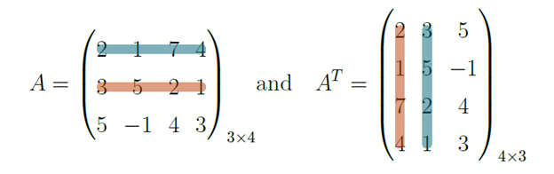
Let’s say B is the resultant matrix from the multiplication of A by A^T. B has dimensions of 3 × 3. The element b_1,2 is the dot product between the vectors highlighted in blue, and the element b_2,1 is the result of the dot product between the orange highlighted vectors. The result of these dot products is equal. The vectors are the same in the two operations, therefore b_1,2 = b_2,1. This result will occur for every element of these matrices except for the diagonal since the diagonal comes after the dot product between two equal vectors. The first step of getting the three components of the SVD for the equation, A = U ⋅ Σ ⋅ V ^T, is done: now we will multiply both sides by A^T:

T T T T A ⋅ A = (U ⋅ Σ ⋅ V ) ⋅ U ⋅ Σ ⋅ V

There are a lot of T′s in that equation, but as we have diagonal and orthonormal matrices, we can make the equation look a little better. It follows that (A ⋅ B)^T = B^T ⋅ A^T, and if we apply this to the equation, it becomes:

AT ⋅ A = V ⋅ ΣT ⋅ U T ⋅ U ⋅ Σ ⋅ V T

Okay, so I have two pieces of information about these matrices that will allow some further simplification:

That guy, Σ is a scaling matrix and therefore a diagonal matrix. The only non-zero entries are on the diagonal, and therefore the transpose is equal to the original matrix, i.e, Σ = Σ^T.
The matrix U is orthonormal, and it was proved earlier that the transpose of matrices with this property are equal to the inverse: U⁻¹ = U^T.

It follows that:

AT ⋅ A = V ⋅ ΣT ⋅ U T ⋅ U ⋅ Σ ⋅ V T

And the multiplication of U^T by U will result in the identity matrix such that:

AT ⋅ A = V ⋅ Σ ⋅ Σ ⋅ V T

Which is equivalent to:

AT ⋅ A = V ⋅ Σ2 ⋅ V T

(5.8)

We are getting closer to a way to compute V , which is not bad, but we still don’t know how to get Σ or U. The problem is that we are depending on Σ to compute V . Our solution is to fetch something that we learned earlier and then to apply it to see if we can make some progress. Looking at 5.8, we know that Σ² is full of scalars on its diagonal, and, just to satisfy your curiosity, they are all positive. The only equation I can recall that we’ve covered lately with scalars on the diagonal of a matrix is the one we used to compute eigenvalues. Let’s see if something can be done with this, but allow me to refresh your memory:

−→ −→ A ⋅ v = λ ⋅ v

(5.9)

Let’s try to make equation 5.8 look similar to equation 5.9. For that, we need a vector or another matrix on the right side. We know that V ^T = V ⁻¹ and we can leverage this by multiplying 5.8 by V on both sides:

T 2 − 1 A ⋅ A ⋅ V = V ⋅ Σ ⋅ V ⋅ V

And, it follows that:

AT ⋅ A ⋅ V = V ⋅ Σ2

(5.10)

Take a good look at this bad boy. Sometimes mathematics is almost like an illusion. Let’s say that A is equal to A^T ⋅ A, then V takes the place of −→v , and the matrix which just has elements on its diagonal replaces λ. This means we have created an eigenvalue problem where Σ is an eigenvalue matrix. Okay, we can work with this! So, we have found a way to compute Σ and V , but we still need U. I multiplied A on the left by A^T, and all the U’s went for a walk: they disappeared from the equation. So perhaps I can multiply A by A^T, but this time on the right. And who will be taking a walk this time? That’s right; it will be the V ’s. Let’s check:

A ⋅ AT = U ⋅ Σ ⋅ V T(U ⋅ Σ ⋅ V T)T

I think you can see where this is going. We do the same as we did before when we computed the equation by multiplying A by A^T on the right:

A ⋅ AT = U ⋅ Σ ⋅ V − 1 ⋅ V ⋅ Σ ⋅ U T

Then:

A ⋅ AT = U ⋅ Σ2 ⋅ U T

And multiplying by U on both sides, it follows that:

T 2 A ⋅ A ⋅ U = U ⋅ Σ

(5.11)

We end up with a similar eigenvalue problem, and Σ happens to be the same for the two equations. Solving these eigenvalue equations will give us U and V . And as A ⋅ A^T is a square symmetric matrix, its eigenvalues will all be distinct and real; when squared rooted, they will give us the single values. The eigenvectors that form U and V will be orthogonal, allowing any vectors transformed by these matrices to preserve the angles between them. If we recall the ”requirements” for all those transformations when done graphically, this was exactly it. There is only one more thing, the matrix Σ which contains the single values will be sorted such that, σ₁ ≥ σ₂ ≥ … ≥ σ_n.

I believe that the computation of such matrices will become solidified for you with a simple numerical example. Consider the matrix A defined as:

( ) ( ) | 1 0 | | 1 − 2 0| | | A = | | and AT = | − 2 − 2 | ( 0 − 2 1) || || ( 0 1 )

(5.12)

The first step will be to compute A.A^T and A^T.A:

( ) ( ) 1 0 ( ) 1 − 2 0 | | 5 4 | | || − 2 − 2|| | | A ⋅ AT = | 0 − 2 1 | . | | = | 4 5 | ( ) | 0 1 | ( ) ( )

( ) ( ) 1 0 ( ) 1 − 2 0 | | 1 − 2 0 | | | − 2 −|2 | | | − 2 8 −|2 AT ⋅ A = || || . | 0 − 2 1| = || || | 0 1| ( ) | 0 − 2 1| ( ) ( )

To compute the matrix U, we need to solve the eigen problem in equation 5.11, let’s start:

| | | | |5 − λ 4 | T || || 2 det(AA − λ ⋅ I) = | 4 5 − λ| = λ − 10λ + 9 || ||

= (λ − 9)(λ − 1)

This results in λ₁ = 9 and λ₂ = 1. Now we need the eigenvectors:

T −→ −→ AA u = λ u

For the value of λ₁ = 9 it follows that:

( ) ( ) | − 4 4| | u1|1 | | .| | = 0 ( 4 −)4 ( u1)2

That, in turn is equivalent to:

{ { − 4u11 = − 4u12 ⇔ u11 = u12 4u11 = 4u12

So we have u₁₁ = 1 and u₁₂ = 1 meaning that −→u1 = (1, 1)^T. Remember that U is an orthonormal basis. Its vectors must have length 1. We need to normalise them. Let’s start by calculating ’s norm:

√ ------ √ -- ∥u1 ∥ = 1 + 1 = 2

So u₁ is such that:

( ) 1 | √2-| −→ | | u1 = | √1-| ( 2)

Doing the same for the eigen value, λ = 1:

( ) ( ) | 4 4| | u2|1 | | .| | = 0 ( 4 4) ( u2)2

With:

{ { 4u21 = − 4u22 ⇔ u21 = − u22

In this case we have found that u₂₁₁ = −1 and u₂₂ = 1, meaning that −→u 2 = (−1, 1)^T. The norm of is also √ -- 2 , therefore the normalised form of −→ u2 is:

( ) √1- | − 2| −→u = | -1- | 2 |( √2- |)

Perfect, so we have computed the matrix U. It is an orthonormal matrix because the eigenvectors have been normalized and A^T.A is a symmetrical matrix. Its eigenvectors are therefore orthogonal:

( ) 1√-- − 1√-- U = ( 2 2) 1√-- 1√-- 2 2

Next, we need the eigenvalues of A ⋅ A^T:

| | ||1 − λ − 2 0 || | | det(AT A − λI ) = | − 2 8 − λ − 2 | || || | 0 − 2 1 − λ|

= (1 − λ) [(8 − λ )(1 − λ) − 4] − 4(1 − λ ))

2 = (1 − λ ) (8 − λ) − 8(1 − λ)

= (1 − λ )(8 − 9λ + λ2 − 8)

= λ(1 − λ )(λ − 9)

Thus, it follows that, λ₁ = 9, λ₂ = 1 and λ₃ = 0. And to define V , we are just missing the normalised eigenvector for each eigenvalue:

For λ₁ = 9:

( ) ( ) | − 8 − 2 0 | | v11| | | | | | − 2 − 1 − 2| | v12| || || .|| || = 0 ( 0 − 2 − 8) ( v13)

( ( | | || − 8v11 − 2v12 = 0 || − 8v11 = 2v12 ||{ ||{ − 2v11 − v12 − 2v13 = 0 − 2v11 − v12 − 2v13 = 0 | ⇔ | ||| − 2v12 − 8v13 = 0 ||| − 2v12 = 8v13 |( |(

( ( | | |{ − 8v11 = − 8v13 |{ v11 = v13 | − 2v11 − v12 − 2v13 = 0 ⇔ | − 2v11 − v12 − 2v11 = 0 |( |(

( ( | | |{ v11 = v13 |{ v11 = v13 ⇔ | − v12 − 4v11 = 0 | v12 = 4v11 |( |(

For −→ v1 we have the vector (1,−4, 1)^T, and its norm is given by:

∘ -2---------2-----2- √ --- ∥v1∥ = 1 + (− 4) + 1 = 18

This makes the normalised version of −→v 1 equal to:

( ) 1 | √18-| | | −→ | −√-4-| v1 = || 18 || | √1--| ( 18 )

Carrying on with the eigenvalue calculations, for λ₂ = 1, we have the following:

( ) ( ) | 0 − 2 0 | | v21| | | | | || − 2 7 − 2|| .|| v22|| = 0 | | | | ( 0 − 2 0 ) ( v23)

( | ( || − 2.v22 = 0 ||{ ||{ v22 = 0 − 2v21 + 7v22 − 2v23 = 0 | ⇔ | − 2v21 − 2v23 = 0 ||| − 2v22 = 0 |( |(

( | |{ v22 = 0 | v21 = − v23 |(

For −→ v2 we have the vector = (−1, 0, 1)^T and the norm of −→v2 :

∘ ------------- √ -- ∥v2 ∥ = ( − 1)2 + 12 = 2

So the normalised version of −→ v2 is:

( 1 ) − √2- || || −→ | 0 | v2 = | | |( √1- |) 2

Finally, −→ v2 , where λ₃ = 0, is:

( ) ( ) | 1 − 2 0 | | v31| | − 2 8 − 2| | v | || || .|| 32|| = 0 | 0 − 2 1 | | v | ( ) ( 33)

( | ( ||| v31 − 2v32 = 0 | |{ |{ v31 = 2v32 − 2v31 + 8v32 − 2v33 = 0 | ⇔ | 2v32 = 2v33 ||| − 2v32 + v33 = 0 |( |(

( | |{ v31 = 2v32 | v31 = v33 |(

For −→ v3 we have the vector (2, 1, 2)^T, and its norm is equal to:

∘ -2-----2-----2 √ -- 2 + 1 + 2 = 9 = 3

Which makes the normalised version of −→v 3 :

( ) 2 | 3| −→ || 1|| v3 = | 3| | 2| ( 3)

The only matrix we’re missing is Σ, but in fact, we have all the information we need to populate this matrix because the σ´s are the square root of the eigenvalues, so σ_i = √ --- λi :

( ) | 3 0 0| Σ = | | ( 0 1 0)

That was quite a bit of work, but thankfully we have computers, so it’s not necessary to do this every time you wish to apply this algorithm. All the same, I believe that going over a simple example is always helpful to solidify your understanding of the algorithm in full. There’s also the added bonus that these three matrices will allow you to do several things, so understanding how they are derived and what constitutes each is a great piece of knowledge to add to your arsenal. Finally, we can represent A as:

( ) ( ) √1-- − √-4- √1-- ( ) | 18 18 18| √1- − √1- | 3 0 0 | | − √1- 0 1√--| U ΣV T = ( 2 2 ) ⋅| 0 1 0 | ⋅ || 2 2 || √1- √1- ( ) | 2 1 2 | 2 2 2×2 ( 3 3 3 ) 2×3 3×3

We should check that I’m not just talking nonsense or making shit up! Every time I use a sauna, I think about something similar. What if the guy that invented this concept of a room that gets really warm and steamy was just messing with us, and now everybody thinks it’s great? To avoid this kind of train of thought, let’s multiply those three matrices:

( ) ( ) √-1- − √4-- √1-- 3√-- − 12 0 | 18 18 18 | || 2 || || − √1- 0 √1- || = | 3√-- 1 0| .| 2 2 | ( 2 2 ) | 2 1 2 | ( 3 3 3 )

( ) 1 − 2 0 || || = ( 0 − 2 1) = A

In the example we’ve just covered, we computed the full version of the single value decomposition, which implies that both the null and left nullspaces are part of the matrices V ^T and U. Previously, we concluded that the nullspace would be in the rows of matrix V ^T. The equation that allowed us to compute the eigenvector for an eigenvalue of 0 is the same as the one we defined for calculating the nullspace: A −→ v = 0. But what about the left nullspace? Well, as a result of the decomposition, I can tell you that this is (0, 0), but let’s verify this. We know that the left null is:

( ) 1 0 ( ) ( ) | | x 0 −→ || − 2 − 2|| | 1| | | AT ⋅x = 0 ⇔ | | ⋅| x | = | 0| | 0 1 | ( 2) ( ) ( )

If we solve that system, we end up with:

( || ||| x1 = 0 || { − 2x1 − 2x2 = 0 ||| || x2 = 0 ||(

As expected, the left nullspace is the vector (0,0), and its dimension is zero. Therefore, if we wish to use the reduced decomposition version, we need to remove the nullspace from the matrix V and adjust the matrix Σ accordingly:

( ) ( ) ( ) -1-- --4- --1- -1- -1- 3 0 | √18 − √18- √18-| T ( √ 2 − √ 2) || || | 1 1 | Ur ΣrV r = 1 1 ⋅ ( 0 1 ) ⋅ |( − √2- 0 √2-|) √2- √2- 2×2 2×2 2×3

This is a lot of mathematical contortions: rotations, stretches, and equations. Next, I’ll present a small example of a real-life scenario where the decomposition of matrices is an excellent way to extract practical, valuable information. But before that, I would like to point out that the single value decomposition includes nearly everything we’ve learned so far in this book: it is thus an excellent way for us to make a self diagnosis on the solidity of our understanding of the linear algebra concepts that have been presented.

On the theme of applicability, I believe that there are three main areas in which to use SVD. The first one, my favourite, is the creation of latent variables. These are hidden relationships that exist within data. An elementary example would be for me to predict if it was raining or not without information on the weather report. For instance, I could do so by observing whether your jacket is wet or not when you arrive home.

I can also discuss an example where I produced great results when trying to predict outcomes related to human emotions, all by analysing hidden variables. It’s hard to have a data set containing a happiness feature from the get-go, but perhaps these can be extracted from the data as a latent variable. With SVD, these variables are present in the matrices U and V . These types of variables also allow us to reduce the dimensionality of a data set.

Secondly, the singular value decomposition allows us to make an excellent approximation of a matrix. An approximation can be helpful for two purposes: we can remove data or information that is not relevant to what we are trying to do, making a prediction, for example; and we can condense this approximation to a few vectors and scalars, which can be extremely useful for storing data more efficiently.

Lastly, you can build a simple recommendation system. As this is linear algebra and the focus of this book is to visualise concepts in order to understand how they work, I will illustrate all of the applications described above in a real-world example. Let’s consider a matrix containing item ratings by users. Each user can rate a given item with an integer score that ranges from 1 to 5. A matrix is an excellent choice to represent these dynamics. Let’s say we have six items and we’ll say they are songs. Yep, six different songs that users have rated according to their preferences, and our sample has eight users. Now yes, I know, this is a tiny, tiny data sample. And yes, you are likely to encounter far bigger data sets when the time comes to apply a single value decomposition, but for illustration purposes, this is enough. Let’s then construct this matrix:

song song song song song song ( 0 1 2 3 4 5) user0 1 2 3 4 1 5 user | 4 1 0 3 5 1 | 1| | user2 || 3 0 1 2 2 4 || user3 | 0 2 1 0 1 5 | A = || || user4 | 0 3 1 3 4 1 | user5 | 2 1 1 4 2 3 | |( |) user6 0 4 1 4 0 3 user7 5 0 3 0 1 5

(5.13)

The matrix A is defined by 5.13. Now we need to decompose this into UΣV ^T, but this time I will use a computer to calculate the full version of the SVD. A will then be decomposed into:

T A8 ×6 = U8 ×8 ⋅ Σ8 ×6 ⋅ V6×6

It follows that the matrix U has the following entries:

( context1 context2 context3 context4 context5 context6 context7 context8 ) user − 0.45 0.03 − 0.34 − 0.26 − 0.13 − 0.55 0.02 − 0.52 0 user1 || − 0.35 0.17 0.70 0.08 0.06 0.26 − 0.13 − 0.49 || user2 | − 0.35 − 0.23 0.14 − 0.06 − 0.46 0.17 0.71 0.19 | || || U = user3 | − 0.27 − 0.15 − 0.37 0.72 − 0.28 0.25 − 0.25 − 0.10 | user4 | − 0.28 0.51 0.13 0.44 0.21 − 0.45 0.18 0.39 | || || user5 | − 0.36 0.12 0.07 − 0.36 − 0.37 0.04 − 0.57 0.48 | user6 ( − 0.32 0.37 − 0.42 − 0.23 0.42 0.55 0.16 0.02 ) user7 − 0.38 − 0.68 0.09 0.00 0.55 − 0.10 − 0.09 0.19

For a full version of V , we have:

context context context context context context song ( − 0.361 − 0.28 2 − 0.263 − 0.464 − 0.35 5 − 0.626) song0 − 0.46 0.45 − 0.20 0.54 0.28 − 0.41 song1|| 0.55 − 0.31 − 0.19 0.00 0.61 − 0.44 || V = song2|| − 0.28 0.33 − 0.10 − 0.66 0.56 0.23 || song3|( 0.40 0.64 0.42 − 0.24 − 0.20 − 0.40 |) song4 0.34 0.34 − 0.82 − 0.02 − 0.27 0.17 5

Finally, Σ is equal to:

( ) 15.72 0 0 0 0 0 | | | 0 6.82 0 0 0 0 | | 0 0 6.38 0 0 0 | || || | 0 0 0 3.13 0 0 | Σ = || 0 0 0 0 1.8 0 || | | | 0 0 0 0 0 1.71| || || | 0 0 0 0 0 0 | ( 0 0 0 0 0 0 )

The first thing to notice is that these are three big-ass matrices! I don’t know if it is the coffee I just drank or the size of these bad boys, but this is giving me anxiety! While there is a lot of information to deal with, we’ll take it step by step. We can deduce the values for Σ via an eigenvalues problem, meaning that if we multiply U and Σ, we will end up with the projections of all the vectors −→ u ’s into the newly transformed axes; remember that each of the −→u vectors are orthonormal. And, if we constructed Σ in a way such that σ₁ ≥ σ₂ ≥ … ≥ σ_n, then it makes sense to assume that the highest sigma value will be the furthest point projection. This will therefore represent the biggest spread and hence the highest variance. Let’s define a measure of energy as:

∑n σ2 i i=1

We can then select how much of it to use. Say for example, that we need around 95% of this energy, it then follows that the total energy for our system is equal to:

∑ 6 σ2i = 350.30 i=1

If we wish to use that percentage value, we can remove the values of σ₄, σ₅, and σ₆. Well now, this means two things: we can replace these sigma values with zeroes, which will result in a trio of new U, Σ and V ^T matrices, and consequently a new version of A; and if σ₄, σ₅, and σ₆ become zero, then the matrix Σ has the following format:

( ) | 15.72 0 0 0 0 0| | 0 6.82 0 0 0 0| | | || 0 0 6.38 0 0 0|| | 0 0 0 0 0 0| Σ = || || | 0 0 0 0 0 0| | 0 0 0 0 0 0| || || | 0 0 0 0 0 0| ( 0 0 0 0 0 0)

Essentially, we are just keeping the information represented by the first three singular values, meaning that we will reduce everything to three dimensions, which in machine learning is called dimensionality reduction. We get rid of some information to make our lives easier. In this example, I wish to represent these relationships visually, as the new contexts are very important. These are the so-called latent variables, which define those cunningly hidden relationships in data.

The interpretation of these variables is up to you and it’s usually linked to the nature of the problem that you are dealing with. In this case, the context is the music genre. I should point out that there are other applications for dimensionality reduction. For example, clustering algorithms tend to work better in lower dimensionality spaces. Working with a model with all of the available information does not guarantee good results. But, often, if we remove some noise we will improve the capacity of the model to learn.

What results from this reduction is a new version of the three amigos U, Σ ,and V ^T, which we call the truncated single value decomposition. This version of the decomposition is represented by:

˜A = U ⋅ Σ ⋅ V T m×n m×t t×t t×n

In this case, t is the number of selected singular values, which for this particular example is:

A8 ×6 = U8 ×3 ⋅ Σ3 ×3 ⋅ V T 3×6

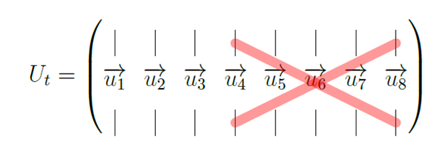
For the truncated version of U, U_t, we can remove the vectors −→ u ₄ to −→u ₈ because we replaced σ₄ to σ₆ with zero. The truncated version of U has the following shape and entries:

truncated U with highlights

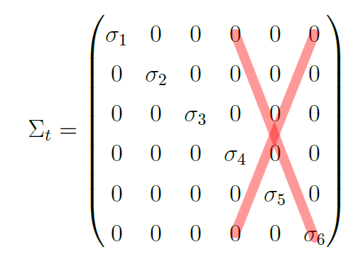
We can apply the same logic to the matrix Σ because the columns will just be zeros after we replace the single values with zeros. We can therefore remove them:

truncated version of sigma

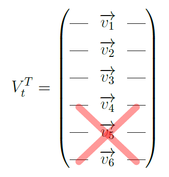
And V ^T will follow:

truncated version of transpose of V

So, U_t is a matrix of users by context:

( context1 context2 context3 ) user − 0.45 0.03 − 0.34 0 user1 || − 0.35 0.17 0.70 || user2 | − 0.35 − 0.23 0.14 | || || Ut = user3 | − 0.27 − 0.15 − 0.37 | user4 | − 0.28 0.51 0.13 | || || user5 | − 0.36 0.12 0.07 | user6 ( − 0.32 0.37 − 0.42 ) user7 − 0.38 − 0.68 0.09

In this example, the matrix A contains information about user ratings for different songs, so perhaps one interpretation of this context’s variables could be the song genre: hip hop, jazz, etc. This is just one possibility as the interpretation for this particular type of variable is dependent on the business problem at hand. Now we have another way of relating users, as we go from song ratings to song genre, and we also have a smaller matrix, the matrix U. Because we were able to reduce the dimensions by only selecting the three highest singular values, we can plot this thus:

−−−−−00−00uuuuuuuu..ssssssss00000505eeeeeeee......rrrrrrrr4433550123456755

Figure 5.6: The secret space of the users.

We can identify some patterns in this plot in terms of similarity of taste based on music genre. Specifically, user₀ and user₇ seem to have similar tastes and the same seems to be evident with the pairs of user₂,user₅ and user₆,user₃. It is true that, in this example, you could identify these relationships by simply looking at the matrix A. Still, your matrix will probably have a much higher dimensionality in a real-world situation, and the number of columns will be much larger. With this information, we could segment users based on their music tastes.

An excellent way to do this would be to apply a clustering algorithm to matrix U, as this would return user cohorts who share song preferences. The reason we only use U is that this a fairly simple example and the singular values are not that distinct. In case of higher dimensionalities with singular values that differ more, it would be better to use UΣ. The immediate advantages of this include being able to work in a smaller space. Certain algorithms will perform well in these types of space, and it will be computationally cheaper to train them. I won’t assume that these concepts are familiar to you, so I will briefly explain. A clustering algorithm has the goal of grouping data that shares identical features, in this case, users that are similar to each other. If you were to run it on matrix U, the outcome would probably be comparable to what I described above. The result would be five groups:

Cluster Population 1 user0 and user7 2 user2 and user5 3 user6 and user3 4 user1 5 user4

Now, to train a classifier. Hold on one moment; those are some seriously fancy words that circulate in every meeting room and blog on the internet… if you are completely new to machine learning, “training” means to find a configuration for a set number of parameters that characterise a model or an equation.

Okay, back to the point, to train this you need a particular dataset which has labels. These labels are like an outcome that the features will characterise. So, for example, the metrics of the data can be a set of measurements of an engine, and the label can be whether or not the motor was working, a zero for not working and a one otherwise. An algorithm will then accommodate a set of parameters so that those two classes can be separated. For simplicity, say that our model is a line. The equation for this shape is y = mx + b. We want to build our model in a way that separates our data into two groups. We aim to have as many zeros below the line as possible, and the maximum number of ones above it. The only thing we can control with that line are the parameters m and b.

So, we will try to find a configuration that can separate our data in the best way possible, and for that, we will be using the provided data set. For example, we can start by randomly drawing a line in space. Our goal is to have all of the one labels above the line and all of the zero labels below the line. As we randomly selected values for m and b, it’s likely that these values will not be the best right away but how can we verify this?

Well, this is why we need the labels. We can count the number of ones that are above the line and the quantity of zeros that are below the line. We can then tweak the values of m and b to see if this result has improved, meaning that we have more ones above and more zeros below the line respectively.

1111111001000000

Figure 5.7: An example of separation achieved by a line.

The algorithm I’ve just described will look randomly for solutions; these types of algorithms are generally called “greedy”. It will not be a good heuristic if we don’t tell it where to look for the best solutions. But this is just an example; if you are curious, one way of providing an algorithm with information on where to move is via derivatives.

Such concepts will be part of volume two, which will be a book dedicated to calculus. The point here is to understand that, in order to train a model, we need to get a configuration of parameters for an equation (or several) that allows us to achieve our goal as well as we can. So if we have a dataset with labels, there are times when we can better separate data by using latent variables. As we are reducing the number of columns going from A to U, the process is called “dimensionality reduction” in machine learning. This is because we have moved from a higher dimensional space to a lower one, thus reducing the complexity of our problem. Going back to the example of SVD, we haven’t looked into the information in matrix V . This particular matrix happens to be an interesting one because it will provide us with the relationship between genre and songs:

context1 context2 context3 song0 ( − 0.35 − 0.46 0.54 ) song1 | − 0.27 0.45 − 0.30 | song2 || − 0.26 − 0.19 − 0.19 || Vt = | | song3 |( − 0.46 0.54 0.00 |) song4 − 0.35 0.27 0.60 song5 − 0.62 − 0.41 − 0.44

Similarly, we can plot this to visually check for closer relationships between songs rather than users:

−−−−00−00ssssss..oooooo0000505nnnnnn.....gggggg65435012345

Figure 5.8: Another secret space, the one of the songs.

We can see that song₀, song₃ and song₄ seem to be of the same genre, while song₅, is probably from a different genre. Finally, song₂ and song₁ seem to be from the same or a similar genre.

So, we have identified a use case for the single value decomposition. By computing U and V ^T, we found new hidden relationships in the data, represented by the latent variables. We also learned that we could leverage these relationships to train algorithms. Just by itself, this is extremely useful, but we can do more with this decomposition.

If you recall, a matrix is a linear transformation. When you multiply a vector by a matrix, you will be moving these vectors, a movement that can take place within the same space or between different spaces. In this example, we have two matrices that we can use to transform vectors. These are the matrices U and V ^T. Let’s look into V ^T. This matrix has context for columns, which for us is the same as music genre, whereas the rows are songs. So we went from users and song ratings, via matrix A, into a new space, V ^T which relates songs by genre. We can create a vector with user ratings and transform it with V ^T to understand which genre this particular user is most interested in. Let’s check this with an example. Say that we have user₈ with the following ratings:

user8 = [5, 0, 0,0, 0,0 ]

If we now transform the user₈ vector via the matrix V , we will transform user₈ into a space of songs by context:

( ) | 0.35 − 0.46 0.54 | | | || − 0.27 0.45 − 0.30 || | − 0.26 − 0.19 − 0.19 | | | [5,0, 0,0, 0, 0] ⋅ || − 0.46 0.54 0.00 || | | || − 0.35 0.27 0.60 || | | | − 0.62 − 0.41 − 0.44 | ( )

This results in the following vector:

[− 1.79, − 2.30, 2.74 ]

That new vector shows the new context values or the music genres for user₈. With this information, you can, for example, make recommendations. So, you will show this user music from the context or genre 3. It will also be possible to make a user-to-user recommendation, which recommends music from a user with a preferred genre that is similar to user₈. For this, we need a measure of similarity. Let’s refresh our memory and look at one of the formulas we derived when studying the dot product. If you recall, there was a way to compute this metric by making use of angles:

−→ −→ a ⋅ b = ∥a∥ ⋅ ∥b∥ ⋅ cos(𝜃 )

(5.14)

In this case 𝜃 is the angle between the vectors −→a and −→ b . We can manipulate equation 5.14 and leave it as:

−→ −→ --a-⋅--b--- cos (𝜃) = ∥a ∥ ⋅ ∥b∥

(5.15)

Equation 5.15 is the cosine distance, and the intuition here is that the smaller the angle between the vectors, the closer they are to each other. So now you can ask me, why do I need all of this mathematics if I could simply calculate the cosine distance between the new user₈ and the users in matrix A? Trust me, I have a severe allergy to work, and if this was not useful, I wouldn’t put it here. Take, for example, users, 3, 4, and 6. If we calculate the dot product between user₈ and these other users in the space of the matrix A (users by song ratings), we will find that it is equal to 0. They are therefore not similar at all. And, users who don’t have ratings in common can represent a problem. To overcome such situations, we can transform user₈ into the space of songs by context. Now, if we calculate the cosine distance between user₈ contexts or genre values and the vectors in matrix U, we will get the user or users that are more similar to user₈ in terms of context. It then follows that:

user 𝜃 user0 95.80 user1 48.29 user2 29.01 user3 95.10 user 96.60 4 user 67.90 5 user6 123.50 user7 37.51

We are looking for the smallest angle value, as this dictates the proximity between vectors (and similarity between users). With this in mind, we can see that the users who are more similar to user₈ are user₇ and user₂. We could therefore recommend a highly-rated song from these users to user₈ if user₈ have not yet rated it. One more useful thing that comes from the single value decomposition equation is that it can represent a matrix as a sum of outer products:

t ∑ −→ −→ A = σi ⋅ui ⊗ vi i=1

In this equation t is the number of single values selected for the approximation. Graphically, this equation has the following shape:

σu⊗v+σu⊗v111666 ...+

Figure 5.9: A new way to represent a matrix.

This means we can create approximate versions of the matrix A by selecting different numbers of single values, just like the truncated version of the SVDs. Let’s see what happens if we choose to approximate A with the first single value. For −→u 1 , we have the vector:

−→ u1 = (− 0.45, − 0.35, − 0.35, − 0.27, − 0.28, − 0.36, − 0.32, − 0.38 )T

The vector −→v 1 is :

−→v = (− 0.35, − 0.27, − 0.26, − 0.46, − 0.35, − 0.62 )T 1

Finally, for σ₁, we have the scalar 15.72. An approximation of A with only a single value will be named A₁^∗; it can be represented by:

A ∗= σ ⋅ −→u ⊗ −→v 1 1 1 1

It follows that:

( ) | 2.55 1.98 1.84 3.26 2.48 4.39 | | | | 1.98 1.54 1.43 2.54 1.93 3.42 | || || | 1.98 1.54 1.43 2.53 1.92 3.41 | || || | 1.55 1.21 1.12 1.98 1.51 2.68 | A ∗ = | | 1 || 1.64 1.27 1.18 2.09 1.59 2.82 || | | || 2.06 1.60 1.48 2.63 2.00 3.55 || | | | 1.85 1.44 1.33 2.36 1.80 3.18 | || || ( 2.19 1.70 1.58 2.80 2.13 3.78 )

This is not a very good approximation as A is:

( ) | 1 2 3 4 1 5| | | | 4 1 0 3 5 1| || || | 3 0 1 2 2 4| || || | 0 2 1 0 1 5| A = | | || 0 3 1 3 4 1|| | | || 2 1 1 4 2 3|| | | | 0 4 1 4 0 3| || || ( 5 0 3 0 1 5)

Let’s see what happens if we consider two singular values instead of one:

A ∗ = σ ⋅ −→u ⊗ −→v + σ ⋅ −→u ⊗ −→v 2 1 1 1 2 2 2

In this particular case, A₂^∗ seems to be a better approximation for A, which makes sense:

( ) | 2.44 2.09 1.80 3.39 2.55 4.30 | | | | 1.43 2.10 1.19 3.20 2.28 2.92 | || || | 2.71 0.83 1.75 1.67 1.48 4.06 | || || | 2.06 0.72 1.34 1.40 1.21 3.13 | A ∗= | | 2 || 0.04 2.85 0.49 3.98 2.57 1.39 || | | || 1.68 1.98 1.33 3.08 2.24 3.21 || | | | 0.69 2.58 0.83 3.74 2.51 2.15 | || || ( 4.35 − 0.40 2.52 0.28 0.82 5.71 )

To verify if this is the case, we will make use of a norm, a measure of distance, called the “Frobenius norm”, as in the following formula:

┌ ----------------- │ m n │ ∑ ∑ 2 ∥A ∥F = ∘ | aij | i=1 j=1

If we calculate this norm for the differences between the matrix approximations and matrix A, it will provide a good idea of which is closer to A:

∥A − A ∗∥ = 10.17 and ∥A − A ∗∥ = 7.54 1 F 2 F

Why is this useful? Well, one purpose can be to store a vast matrix. For example, suppose you have a matrix of 1 million rows by 1 million columns and you choose to approximate it using the most significant singular value. In that case, it is only necessary to store two vectors of size ten and one scalar (the single value).

Before wrapping up, I would next like to introduce one more technique we mentioned at the start of this book that is widely used in machine learning.