Introdução à Matemática Linear

What About a Matrix?

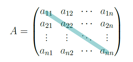
A matrix is a rectangular arrangement of numbers, symbols, or functions organized in rows and columns. In various contexts, a matrix may denote a mathematical object or an attribute of such an object. A key feature of these elements is their order or size, defined by the number of rows and columns. Matrices are commonly denoted by capital letters, and can be represented using the following notation:

A m ×n

In this representation, m is the number of rows and n is the number of columns. An example of a 3 × 3 matrix is:

( ) 1 4 12 || 9 5 1 || A3 ×3 = ( ) 8 2 7

If we wish to generalise a representation for all matrices, we can rewrite the one above in a form that will accommodate any case:

( a a ⋅⋅⋅ a ) 11 12 1n || a21 a22 ⋅⋅⋅ a2n || A = | .. .. ... .. | m ×n | . . . | ( am1 am2 ⋅⋅⋅ amn )

The a′s are referred to as an entry, with each of these being defined by their index. For instance, a₁₁ is the element in the first row and the first column of the matrix. In machine learning, the use of matrices mainly accommodates three different cases. Let me explain.

4.1 When a Table Isn’t Furniture

There is one element without which we would be unable to do any work with machine learning algorithms; features. Features are what characterise your data. They are a set of metrics per element of granularity, from which your algorithm will try to learn signals. This same set can be represented as a vector, and, if you combine all the vectors into a single structure, you end up with a matrix. For example, say that we wish to predict whether a student will make it onto the basketball team based on their weight, height, and an average of their grades (assuming that their grades are a real number). Here the granularity, a word that reflects the level of detail present in the data, is the students, and the metrics are height, weight, and the average grade. Students can be represented by vectors:

Student1 = (1.65, 64, 5) Student2 = (1.54, 67, 4) ... Studentn = (1.61, 55, 2)

Combining these vectors will produce a feature space matrix that can be placed alongside a target variable. An example of such a variable is a Boolean indicator; that’s just a fancy name for a variable that can only take two values, for example, yes or no. This variable will then exhibit whether or not a student made it onto the basketball team. This enriched data set can then be used to perform predictions:

( ) 1.65 64 5 yes || 1.54 67 4 yes || | ... ... ... ... | |( |) 1.61 55 2 no

4.2 Yoga for Vectors – Linear Transformations

The second representation of a matrix is a linear transformation. Bear with me; this is a concept that has the potential to change your learning experience of linear algebra. As this notion is related to movement in space, we can showcase it using visualisations. This will help to solidify a deep understanding of an idea that, although simple, is essential when it comes to understanding everything else in this book. It is an excellent tool to have in your arsenal, and it includes most of the techniques already studied.

Breaking down the term will give a pretty good indication of what we are dealing with. In fact, this is good practice in mathematics. After all, the names have to make some kind of sense. Actually, for a long time these names did not make sense to me because I always associated them with a formula, and never stopped to think about what the names truly meant. This cost me time, but for some reason, one random day, it clicked. I remember with which one it was, the standard deviation. I was walking along, and all of a sudden, almost like an epiphany, everything was clear in my mind. Standard deviation is how much data deviates from the standard. But what is the standard? Probably the mean. Following the happiness of this moment, one of the best sequences of letters (that works like a charm in the right situation) came to me out loud; Motherfucker!

Now, we have covered the meaning of the word linear: no curves please, so all lines will remain lines. Transformation is another word for mapping or function. Also, is it important to mention that, despite the tasks in hand, the origin of the vectors must remain intact in transformations. So we will be transforming vectors into vectors or scalars via matrices. Analytically, a linear transformation L between two spaces Z and R can be represented as:

L Z → R

The vector is going from Z to R via L. More rigorously, a linear transformation L is defined as:

L : Z → R

Since we are not gonna be considering any complex numbers in this book, we can even be a bit more particular and define the linear transformations as:

L : ℝn → ℝm

This means we will move a vector from a space with n dimensions into a space with m dimensions. For the purpose of demonstration, let’s consider n = m = 2. I can give you an ego booster here; when n = m, the linear transformation is called an endomorphism. Don’t say I am not your friend, dropping all these fancy names.

We are defining a way to move a vector in space via patterns that allow it to keep its origin, but also to rotate and/or stretch. The transformation defined by L will map every vector in the same way. In the following example, L is a 180 degree rotation of any vector from the vector space ℝ²:

xy−−234−−−1234IOLnu43432ptuptutvecvteocrtor

Figure 4.1: An example of a linear transformation.

The plot bellow, is to showcase the fact that a linear transformation will do the same thing to every vector that we decide to map:

−→−−→−→−→−→−→−→→ xy−−−1234−−−234wwzyxz∗y∗x∗432432∗

Figure 4.2: Some mappings via the same linear transformation.

This transformation is defined by:

L : ℝ2 → ℝ2

(l1,l2) → (− l1, − l2)

The letters, l₁,l₂ represent generic coordinates of a given vector, for example, given any vector −→v ∈ ℝ², with coordinates (v₁,v₂) the linear transformation L will transform the coordinates of this vector into their negations, (−v₁,−v₂). Negation is not a depreciative term. It means the negative version of a positive number, or vice versa, and numbers do not have feelings, well, so far. Analytically, we have defined linear transformations, but we have yet to understand why we need matrices for these functions. To do so, let’s start by considering one basis of ℝ², the one defined by −→ i and −→ j where:

( ) ( ) −→ 1 −→ 0 i = 0 and j = 1

So any vector that belongs to ℝ² can be represented as:

−→ −→ α ⋅ i + β ⋅ j

Which is the same as having:

( ) ( ) 1 0 α ⋅ 0 + β ⋅ 1

(4.1)

Where α,β ∈ ℝ. If you don’t believe me, I will dare you to find a vector that belongs to ℝ² that can’t be obtained by equation 4.1. Let’s make this interesting, I will buy a car for the person that finds out about such a vector. Subscribe to the mailing list to participate in this context. Press Here! (Note: This is a marketing trick, don’t forget to erase this note before printing the book). Now, let’s grab a vector −→v ∈ ℝ² and write it down as a linear combination of −→i and −→j . If we select the values (2, 3)^T as the coordinates of −→ v , it follows that:

−→ −→ −→v = 2 ⋅ i + 3 ⋅ j

(4.2)

We defined L on the fact it will rotate any vector in ℝ² by 180 degrees. If we apply this transformation to the basis −→ i , −→ j and call the resultant vectors as −→ i∗ , −→ j∗ we have:

−→ ( ) −→ ( ) i∗ = − 1 and j∗ = 0 0 − 1

Alright, let’s grab equation 4.2 and replace −→ i and −→ j by −→∗ i and −→∗ j respectively:

−→ −→ −→ v∗ = 2 ⋅ i∗ + 3 ⋅ j∗

Here, −→ v ∗ represents a new version of −→v which is defined as a linear combination of the transformed base. It follows that:

( ) ( ) ( ) −→ − 1 0 − 2 v ∗ = 2 ⋅ + 3 ⋅ = 0 − 1 − 3

Well, −→ v ∗ is the same as −→ − v , meaning that −→ v∗ is the negated form of , exactly like we defined L. As a result, it is possible to represent a linear transformation by adding two scaled vectors:

−→−→−→−→−→−→ xy−−−−234−−2342233vijv∗432143i∗j∗

Figure 4.3: The transformation of both −→v

and its basis.

Generically, if −→ v = (v₁,v₂) is any vector of ℝ², a linear transformation can have the form:

−→ −→ −→ v∗ = v ⋅ i∗ + v ⋅ j∗ 1 2

To transform a given vector from ℝ², we can start by mapping the standard basis. Then, suppose we add the result of multiplying each of the elements of the original vector by the vectors of this transformed version of the basis, respectively. In that case, we will obtain the desired transformed vector. Let’s consider another example to solidify this important concept. Say that we now have G, a linear transformation where −→ i and −→ j are transformed into (2, 1)^T and (1, 2)^T. A vector that results from applying G can be described as −→ ∗ g :

( ) ( ) −→ ∗ 2 1 g = g1 ⋅ 1 + g2 ⋅ 2

(4.3)

We are missing the vector from which we desire to obtain a transformed version, the vector −→ g . Let’s say that g₁ and g₂, the elements of −→g , are equal to 1. Consequently, we have:

( ) g1 (1 ) −→g = ( g2) = 1

So, it follows that:

( ) ( ) ( ) −→ ∗ 2 1 3 g = 1 ⋅ 1 + 1 ⋅ 2 = 3

If you are curious, this is the analytic representation of G:

2 2 G : ℝ → ℝ

(g1, g2) → (2 ⋅ g1 + g2,g1 + 2 ⋅ g2 )

And, visually, this is how we can represent this transformation:

−→−→−→−→−→−→ xy−−−−1234−−−−1234jgii∗j∗∗g43214321

Figure 4.4: The transformation of −→g

Before moving onto a matrix representation of linear transformations, there is something else to cover. We’ve spoken about changing basis, linear transformations, and changing basis with linear transformations. A change of basis is not a linear transformation. You can do a change of basis via an isomorphism, which is a linear transformation between the same spaces. Remember that changing the basis just changes the perspective of the same vector, whereas a linear transformation, as the name suggests, can change the vector; it is a transformation. For example, consider an arbitrary mapping from ℝ² to ℝ³:

2 3 H : ℝ → ℝ

(4.4)

(h1, h2) → (7h1, 2h2 + h1, h1 + h2)

The equation 4.4 can’t represent a change of basis, but a linear transformation sure can. It is true that we did not define the conditions that a mapping has to obey in order for it to be considered linear. But it is Sunday, and I was hoping that you would let this one slide… no? Forward we move then. A linear transformation L : ℝⁿ → ℝ^m must satisfy two conditions:

L( + ) = L() + L()
L(c ⋅) = c ⋅ L()

For all vectors −→v , −→u ∈ ℝⁿ and all scalars c ∈ ℝ. Alright, let’s verify if H satisfies the two conditions above. On H we go from ℝ² to ℝ³ so we can define −→ v and −→ u as (v₁,v₂) and (u₁,u₂). The plan of attack will be to get the left side of the item’s one equation and develop to see if we arrive at the equation on the right of the same item’s number. We need ( −→v + −→u ) which is the same as (v₁ + u₁,v₂ + u₂). Now this specimen will go for a ride via H:

H (v + u ,v + u ) = (7(v + u ), 2(v + u ) 1 1 2 2 1 1 2 2

+ (v1 + u1 ),(v1 + u1) + (v2 + u2 ))

I know that stuff is so ugly that if it could look at a mirror its reflection would walk away, but it is what we have to work with. Now for the second part we need H( −→v ) and H( −→u ) to calculate H( −→v ) + H( −→u ). So:

H (−→v ) = (7v1, 2v2 + v1, v1 + v2 )

On the other hand:

H (−→u ) = (7u1, 2u2 + u1, u1 + u2)

Adding them up results in:

−→ −→ H ( u ) + H ( v ) = (7 (v1 + v2 ),2(v2 + u2) + v1 + u1, v1 + v2 + u1 + u2 )

Which is exactly what we are looking for. Now for item number two, let’s start with H(c −→ v ):

H (cv1, cv2) = (7cv1, 2cv2 + cv1, cv1 + cv2)

= (7cv1, c (2v2 + v1),c(v1 + v2))

= c(7v , 2v + v ,v + v ) 1 2 1 1 2

= cH (v1,v2 )

And that proves point number two! This means that we are assured that H is a linear transformation, and there is the opportunity to learn two more fancy names: for item one we have additivity whereas item two is homogeneity.

I want for us to go back to equation 4.3, where we defined the vector −→ g ∗ via a linear combination.

( ) ( ) −→ 2 1 g ∗ = g1 ⋅ + g2 ⋅ 1 2

There is another way of representing such a transformation; we could do so via a matrix.

( ) 2 1 G = ( 1 2 )

To go from one notation to the other, from analytical to a matrix, is very simple. Each row of the matrix will have the coefficients of the variables of each element of the linear equation above. So, the first row of matrix G is 2, 1 because the coefficients of the first element (2.g₁ + g₂) are two and one. The second line of the matrix follows the same logic. The conclusion is that a linear transformation can also be characterised by a matrix.

We now know about vectors and matrices, but we don’t have a way of operating between these two concepts, and in fact, this is what we are missing. To transform any vector with that matrix G, we need to multiply a vector by a matrix.

4.2.1 Could It Be Love? Matrix and Vector Multiplication

Matrix and vector multiplication can be summarised by a set of rules. A method that is appealing to some people for reasons that I will leave to your imagination. On the other hand, I have a very hard time with such things, so instead of just providing a formula to compute these multiplications, we will deduce it. We are not cooking; we are learning mathematics. You shouldn’t be happy because you have a set of instructions to follow. Save that for your bad-tasting vegan dessert. I am just joking. I know you are all foodies that know more than people that spent half of their lives cooking.

Let’s consider any vector, which we’ll call −→ x (we need a x in a mathematics book, so it was about time!), and a matrix A. There is one consideration to bear in mind when defining matrix-vector products, their dimensions. We can only compute this multiplication when the number of columns in A is equal to the number of rows in or the number of columns in −→x is equal to the number of rows in A. So for any matrix A_m×n we can only compute multiplication with vectors of the order −→x _n×1. We can then represent, A ⋅ −→x as:

( ) ( ) a11 a12 ⋅⋅ ⋅ a1n x1 | a21 a22 ⋅⋅ ⋅ a2n | | x2 | || .. .. .. .. || || .. || | . . . . | .| . | ( am1 am2 ⋅⋅ ⋅ amn ) ( xn )

(4.5)

Time for a confession. The term role model would not have applied to me as a student. Under my name on the attendance report, things were not pretty. This lack of showing up is not something that I am proud of these days. I could have learned way more in university, but everything has its positives and its negatives. I missed a lot of classes, but I never flunked. This is because I developed a strategy. Where and when I took my degree, it was not mandatory to go to class; you could just show up on the exam date, and if you scored more than 50%, the job was done. You can’t fully understand a whole semester of classes a week before the exam. That was an easily reachable conclusion. So now I was seriously debating, how could I pass this exam by not attending classes all the time? In the discipline of mathematics, you tend to encounter a dependence on prior knowledge to understand what will come next. You could see it as a problem, but I chose to see it as an advantage. The things you learned in the first weeks of classes will likely be a basis for more complex deductions, concepts, and theorems. So, if you have a solid foundation but need to get to more complex themes, then with some creativity, inspiration, and maybe a little bit of lady luck on your side, you could… wing it. So my strategy, as time was of the essence when studying for an exam, was to just focus on the basics: everything I needed that allowed me to deduce a concept if required.

I am not advocating for people to do this. The fact that I did not attend classes as often as I should have is the sole reason behind my average grades during my degree. Gladly, this changed during my Master’s. I worked harder. The positive from this is that I always ensure that I understand the basics well, which has also helped me immensely in my career as a mathematician that has the job title of data scientist. Now in this book, is there anything that we can use to do something to a big ass matrix and a vector? Well, what about the dot product? Let’s try it. If we compute the dot product row by row on equation 4.5, we will end up with:

( ) a11 ⋅ x1 + a12 ⋅ x2 + ⋅ ⋅⋅ + a1n ⋅ xn | a ⋅ x + a ⋅ x + ⋅ ⋅⋅ + a ⋅ x | | 21 1 22 2. 2n n | || .. || ( ) am1 ⋅ x1 + am2 ⋅ x2 + ⋅⋅⋅ + amn ⋅ xn

Let’s go back to where we finished the exposition of linear transformations with matrix G:

( ) 2 1 ( ) G2 ×2 = 1 2

And we need a 2 × 1 vector, so let’s put −→ g to work again:

( ) 1 −→ g = ( 1)

If we were to multiply G and −→g :

( ) ( ) ( ) ( ) 2 1 1 2 ⋅ 1 + 1 ⋅ 1 3 ( ) ( ) ( ) ( ) 1 2 . 1 = 1 ⋅ 1 + 2 ⋅ 1 = 3

Given that we used G and −→ g on the example above is not a surprise that if we wish to transform a vector by making use of a linear transformation, we just need to multiply this vector by the matrix. Now, let’s define the matrix for the linear transformation H:

( ) 7 0 | | H = | 2 1 | ( 1 1 )

Alright, let’s do some verifications with −→g :

( ) ( ) 7 0 1 || 2 1|| ( ) .( 1 ) = (7,3, 2) 1 1

The linear transformation H is defined such that the new vector is given by (7h₁ + 0h₂, 2h₂ + h₁,h₁ + h₂) so if we replace h₁ with 1 and h₂ with 1 we end up with the same result (7, 3, 2). Cool stuff! This is another use case for a matrix, the representation of a linear transformation. And on the way to understanding it, we introduced matrix-vector multiplications. If a matrix is a set of vectors and we can multiply a vector by a matrix, what is stopping us from multiplying two matrices? Surely not me. Given two generic matrices A_n×m and B_m×p, actually throw one more into the mix, it is happy hour, let’s say that C_n×p is the result of A ⋅ B, so if:

( ) a11 a12 ⋅⋅ ⋅ a1m | | | a21 a22 ⋅⋅ ⋅ a2m | A = | ... ... ... ... | |( |) an1 an2 ⋅⋅ ⋅ anm

And:

( ) b11 ⋅⋅ ⋅ b1p ⌊ ⌊ ⌋ ⌊ ⌋ ⌋ b11 b1p || b21 ⋅⋅ ⋅ b2p|| | | b | | b | | B = | ... ... ... | = | | 2.1 | ... | 2.p| | |( |) ⌈ ⌈ .. ⌉ ⌈ .. ⌉ ⌉ bm1 ⋅⋅ ⋅ bmp bm1 bmp

Then each column of C is the matrix-vector product of A with the respective column in B. In other words, the component in the i_th row and j_th column of C is the dot product between the i_th row of A and the j_th column of B such that:

cij = ai1 ⋅ b1j + ai2 ⋅ b2j + ...+ ain ⋅ bnj

Visually this is what we will have:

´a1aaaaaaabbbbbb,23412341212121,1,1,1,2,2,2,2,1,1,2,2,3,3

Figure 4.5: Coloured squares to help us with matrix multiplication.

Let’s check a numerical example. Say that A_4×2 is such that:

( ) 2 4 | | | 1 1 | A = | 3 2 | |( |) 1 1

And let’s define B_2×3:

( 1 2 1) B = ( 3 1 2)

Then:

( ) 2 4 | | ( ) | 1 1 | 1 2 1 C = A.B = || 3 2 || .( 3 1 2) ( ) 1 1

( 2 ⋅ 1 + 4 ⋅ 3 2 ⋅ 2 + 4 ⋅ 1 2 ⋅ 1 + 4 ⋅ 2) ( 14 8 10) || 1 ⋅ 1 + 1 ⋅ 3 1 ⋅ 2 + 1 ⋅ 1 1 ⋅ 1 + 1 ⋅ 2|| || 4 3 3 || = | 3 ⋅ 1 + 2 ⋅ 3 3 ⋅ 2 + 2 ⋅ 1 3 ⋅ 1 + 2 ⋅ 2| = | 9 8 7 | | | | | ( 1 ⋅ 1 + 1 ⋅ 3 1 ⋅ 2 + 1 ⋅ 1 1 ⋅ 1 + 1 ⋅ 2) ( 4 3 3 )

It is simply not enough. We are manipulating vectors with dot products and dealing with linear transformations. Something is happening in the vector space, and it shouldn’t go to the Vatican to be kept a secret. Consider:

2 2 Z : ℝ → ℝ

(z ,z ) → (− z + z , 2z + z ) 1 2 1 2 1 2

The matrix that represents the linear transformation Z is:

( ) − 1 1 ( ) 2 1

Transforming the vector −→ g with the linear transformation Z results in:

( ) ( ) − 1 1 1 ( ) ( ) −→∗ 2 1 ⋅ 1 = (0, 3) = gZ

−→−→ xy−1234−1234gZg∗Z11

Figure 4.6: A transformation of −→g

by Z.

Now I will define another linear transformation. We will get somewhere, don’t worry, I haven’t lost my mind. I don’t know how to convince you of this, as I think that everybody that loses their mind will state that same sentence, nevertheless, give me a chance. Let’s say that W is defined such that:

2 2 W : ℝ → ℝ

(w1, w2 ) → (w2, w1 + w2 )

It would be interesting to see what happens to vector −→ g ∗Z if we transform it with W. In other words, we are exploring the idea of composing transformations. We are looking at transforming one vector via a matrix and mapping the resultant element with another matrix. So, we will transform the vector that results from changing with Z via the matrix W:

( ) ( ) 0 1 0 −→ ( 1 1) ⋅ ( 3 ) = (3,3) = g ∗ W

−→−→ xy−1234−1234ggW∗Z∗W11

Figure 4.7: A transformation of −→ g∗Z

by W.

The vector −→ g∗W is no stranger to us. It is the same as the vector we obtained when we introduced the subject of linear transformations and used the mapping G as an example. This did not happen by accident, I fabricated this example to showcase a composition, so let’s multiply the two matrices W and Z:

( ) ( ) ( ) 0 1 − 1 1 2 1 ( ) ( ) ( ) 1 1 . 2 1 = 1 2

This is the matrix that defines the linear transformation G, which means that when we are multiplying matrices, we are composing a transformation. We are transforming a vector in one step instead of two. While two applies to this particular case, you can have as many steps as there are matrices that you wish to multiply. This is a good way of looking at matrix multiplication rather than just thinking of a formula. Now you can see that you are just taking a vector for a ride. Either you do it in steps if you wish to multiply the vector by one of the matrices in the multiplication, and then multiply the result of this by the next matrix and so on. Or you can do it in one go and multiply the vector by the resultant matrix of the multiplication.

Never forget that order matters, oops I forgot to mention it, so let’s introduce some matrix multiplication concepts. Contrary to multiplication with real numbers, multiplying two matrices is not commutative, meaning that if A and B are two matrices:

A ⋅ B ⁄= B ⋅ A

The dimensions of the matrices are also critical, you can’t just multiply any two matrices, just like the case of matrix-vector multiplication. The number of columns in the first matrix must be equal to the number of rows in the second matrix. The resultant matrix will then have the number of rows of the first matrix and the number of columns of the second matrix:

A.B=Cmnm ××m×nm

Figure 4.8: Brown, orange and red so the dimensionality isn’t a pain in the head.

There are several ways to multiply matrices, but as we are dealing with linear mappings (we will also introduce linear systems later), we need to pay attention to the dimensions. Finally, the product of matrices is both distributive and associative when dealing with matrix addition:

A(B + C) = AB + AC
(B + C)D = BD + CD

I feel that we are on a roll here with these concepts of multiplication, so I will take the opportunity to present a new way of representing the multiplication of two matrices, if I may. Let’s consider two generic matrices, A and B:

( ) ( ) a b e f A = ( c d ) and B = ( g h )

If we multiply A and B it follows that:

( ) ae + bg af + bh ( ) A.B = ce + dg cf + dh

We can split this into the sum of two matrices:

( ) ( ) ae af bg bh A.B = ( ce cf ) + ( dg dh)

(4.6)

Right, let’s take a look at matrix ( ) ae af ( ce cf ) , there are a´s, e’s, c’s, and f’s. Don’t worry; we will not be singing songs about the alphabet. Those letters are in the first column of A and the first row of B, and it seems that I just have to multiply each entry of one with each entry of the other:

( ) ( ) a ( ) ae af ( ) e f ( ) c . = ce cf

This technique is called the outer product and it is represented by the symbol ⊗. For some reason, for a while, I would have an anxiety attack every time I saw that symbol on a blackboard at university, and now I understand why I feared the notation. There is no reason to fear an equation. They are the syntax of mathematics, the same way that music has symbols and shapes which form notes and tempos. So in terms of notation, if we have vector −→ v with dimensions n × 1 and vector −→ w with dimensions m × 1, and their outer product is computed as:

( v ⋅ w v ⋅ w ... v ⋅ w ) 1 1 1 2 1 n || v2 ⋅ w1 v2 ⋅ w2 ... v2 ⋅ wn || −→ −→ | .. .. .. .. | v ⊗ w = | . . . . | ( vn ⋅ w1 vn ⋅ w2 ... vn ⋅ wm )

This is an operation between two vectors. But, the reason I chose to introduce it while we are dealing with matrices is: well, the first reason is that the result is a matrix. As for the second reason, we can put this operation into context. Going back to equation 4.6, we divided the multiplication of A and B into a sum of two matrices, and followed this with a new way of computing a matrix via the outer product of two vectors. This technique allows us to represent matrix multiplication as a sum of outer products. The outer product of the vectors (b,d) and (g,h) provides the right side of the summation on equation 4.6, so we can generalise the formula for multiplication of matrices as a sum of dots products:

#col∑umnsA A.B = ColumniA ⊗ RowiB i=1

Where Column_iA is the i_th column of A and Row_iB is i_th row of B. There are several applications for representing matrix multiplication as the sum of outer products. For example, if you have a sparse matrix (a matrix in which most entries are zero) you can speed up the computation taken to multiply two matrices by this representation. Another example is the derivation of an approximation of matrices via matrix decomposition, such as a single value decomposition, which we will cover in this book, so bear with me.

By looking at linear transformations, we had the need to understand several other concepts that while not complicated, were of extreme importance. We went on a ride there with the linear transformations (just like the vectors), and I can tell you that by now, you are most likely capable of understanding any concept in linear algebra. Just think about what we’ve covered so far: vectors, dot products, matrices, linear transformations, outer products, the multiplication of vectors by matrices, as well as matrices by matrices. One cool thing you can do with linear transformations is to transform shapes. For example, you can shrink or extend a square into a rectangle, and with this comes a useful concept in linear algebra, the determinant.

4.2.2 When It’s Not Rude to Ask About Size – The Determinant

Linear transformations are a fundamental concept in linear algebra; they allow the rotation and scaling of vectors in the same space or even into new ones. We can also use this mathematical concept to transform geometric figures, like a square or a parallelogram. If we take a two-dimensional space, such formations can be represented by a pair of vectors and their corresponding projections. Let’s use the standard basis −→ i = (1, 0)^T and −→ j = (0, 1)^T and form a square:

−→−→ xy−123−123ij11

Figure 4.9: First example of the determinant saga.

Following on from this, we can define a linear transformation represented by the matrix:

( ) 2 0 L = ( 0 2 )

Applying the mapping L to −→ i and −→ j will result into two new vectors, −→∗ i and −→∗ j , with values (2, 0)^T and (0, 2)^T respectively. If we plot them alongside their projections, this is what it will look like:

−→−→ xy−23−23ij11

Figure 4.10: Second example of the determinant saga.

Visually, the area of the square formed by the basis vectors quadruples in size when transformed by L. So, every shape that L modifies will be scaled by a factor of four. Now, consider the following linear transformation H defined by:

( 1 ) 2 0 H = ( 0 1) 2

If we apply H to the vectors −→ i and −→ j we will end up with −→∗∗ i and −→∗∗ j with values ( 1 2 , 0)^T and (0, 1 2 )^T:

xy−12−12−→−→ij11

Figure 4.11: Third example of the determinant saga.

In this instance, the area of the parallelogram shrunk by a factor of four. The scalar that represents the change in area size due to the transformation is called the determinant. In the first example, we have a determinant equal to four and the second example has a determinant of one quarter. The determinant is then a function that receives a square matrix and outputs a scalar that does not need to be strictly positive. It can take negative values or even zero. For example, consider the transformation Z such that:

( ) − 1 0 ( ) Z = 0 1

To spice things up a little, and I mean it when I say a little bit. Once upon a time in Mexico, I decided to play macho and asked for a very spicy dish. So let’s say that I and the Mexican sewer system had some rough next few days. Let’s consider two new vectors:

( ) ( ) −→ 3 −→ 1 g = , l = 2 2

−→−→−→ xy−−−−−12345−−234−→ggll∗5432121∗

Figure 4.12: Fourth example of the determinant saga.

The image above represents a determinant with a negative value. It might seem strange as the determinant represents a scaling factor. But, the negative sign indicates that the orientation of the vectors has changed. The vector −→ g was to the right of −→ l and after the transformation, is to the left of . Due to this property, the determinant can also be called the signed area. What we are missing is a formula to compute this bad boy, so let’s consider a generic matrix M:

( ) a b M = ( c d)

The notation for the determinant is det(M) or ∣M∣, and the formula for its computation is:

( ) || || a b |a b| det ( c d ) = ||c d|| = ad − bc | |

(4.7)

Why? It is a fair question. Let’s bring up a plot to understand what is going on. We have been speaking about areas, so a visual should indicate why the formula is as shown above:

aabbabbacddcxyccbd2ccbd2∕∕22

Figure 4.13: The geometry of a 2 × 2 determinant.

The quest now is for the area of the blue parallelogram. At first glance, it does not seem like a straightforward thing to compute, but we can find a workaround. We can start by calculating the area of the big rectangle, formed by (a + b) and (c + d), this can be found by (a + b)(c + d). We don’t know the area of the blue parallelogram, but we know that of the shapes around it: four triangles and two squares. So, if we subtract the sum of these from the big rectangle, we end up with the area value of the blue parallelogram. The two brown triangles each have an area of bd 2 , which when summed is bd, so we need to remove bd from the big parallelogram. The two pink squares are each of size bc, which when summed equates to a value of 2bc. And finally, the green triangles are each of size ac 2 , adding them will result in a magnitude of ac. If we sum each of these areas, we arrive at an expression for the value that we need to subtract from the big rectangle area:

| | ||a b || |c d |= (a + b)(c + d) − ac − bd − 2bc = ad − bc || ||

Alright, let’s check what happens if we apply equation 4.7 to the linear transformation Z:

| | |− 1 0| || || | 0 1| = − 1 ⋅ 1 − 0 ⋅ 0 = − 1 | |

This means that the resultant area of a shape transformed by Z will remain the same, but the orientation of the vectors will change, just as we saw in the plot above. If we have a higher dimensionality than two, we will be scaling volumes instead of scaling areas. Consider a generic 3 × 3 matrix, N such that:

( ) a b c | | N = | d e f | ( g h i )

Graphically, the determinant will reflect the change in volume of a transformed parallelepiped:

−→−→−→−→−→−→ xyijkNxyijk∗∗∗

Figure 4.14: The geometry of a 3 × 3 determinant.

Before jumping into the derivation of the formula to compute a 3 × 3 determinant, I would like to introduce three properties of this algebraic concept:

If we have pair of vectors that are equal, its follows that det(,,) = 0. Graphically we can prove this. For example, if we collapse into , we understand that the parallelepiped will also collapse and become flat.
If we scale the length of any side of the parallelepiped, we will also scale the determinant, det(a ⋅,,) = a ⋅ det(,,), where a ∈ ℝ.
The determinant is a linear operation, det(+,,) = det(,,) + det(,,).

These properties are valid for any dimensionality of a geometric shape that we wish to calculate a determinant for, but for now, I would like to do an experiment and use one of these properties to produce the same formula that we have for a matrix of size 2 × 2. For this, let’s formulate the calculation of a determinant such that:

( ( ) ( ) ) a b ( ( ) ( ) ) det (M ) = det c , d

We can represent these vectors as a linear combination of the standard basis vectors −→ i , −→ j :

−→ −→ −→ −→ det(a ⋅ i + c ⋅ j ,b ⋅ i + d ⋅ j )

(4.8)

I feel that there are a ton of letters and no numbers, and I don’t want to scare you off, so let’s do a verification:

( ) ( ) ( ) 1 0 a a ⋅ + c ⋅ = 0 1 c

There! Some numbers to ease us into what’s about to happen. We can make equation 4.8 look more friendly by leveraging property numero tres:

det(a ⋅ −→i , b ⋅ −→i + d ⋅ −→j ) + det (c ⋅ −→j ,b ⋅ −→i + d ⋅ −→j )

This can also be made a bit simpler:

−→ −→ −→ −→ det(a ⋅ i ,b ⋅ j ) + det (a ⋅ i ,d ⋅ j )

−→ −→ −→ −→ +det (c ⋅ j ,b ⋅ i ) + det (c ⋅ j ,d ⋅ i )

Now, by property two we can take those scalars out:

−→ −→ −→ −→ ab ⋅ det ( i , i ) + ad ⋅ det( i , j )

(4.9)

−→ −→ −→ −→ +cb ⋅ det ( j , i ) + cd ⋅ det( j , j )

OK, we can do something with this. If a matrix has identical vectors for columns, it follows that the determinant value is 0. So, ab⋅det( −→ i ,) = 0 and cd⋅det( −→ j ,) = 0. The only two things that are missing are the values of det(,) and det(,). This will be the same matrix, but with switched rows. Let’s see what happens to the determinant when we do such a thing:

| | ||1 0|| |0 1| = 1 ⋅ 1 − 0 ⋅ 0 = 1 || ||

And:

| | |0 1| || || |1 0| = 0 ⋅ 0 − 1 ⋅ 1 = − 1 | |

So, equation 4.9 is equal to:

ad − cb

Which is what we found when we made the geometric deduction. I included this because we can do the same kind of exercise for a matrix with dimension 3 × 3, for example, the matrix N. This time I will save you from all the intermediate steps (as they are very similar to those for two dimensions) and I’ll provide you with the final result:

det (N ) = aei + bf g + cdh − ceg − bdi − af h

(4.10)

We can reorganise the equation 4.10 to:

det (N ) = a(ei − f h) − b (di − f g) + c(dh − eg )

(4.11)

And we can also produce a less condensed version of equation 4.11:

|| || || || || || |e f| |d f | |d e | det(N ) = a ||h i|| − b ||g i||+ c ||g h || | | | | | |

(4.12)

Which has the following graphical representation:

Figure 4.15: Green and yellow for the calculations to be mellow.

For any matrix with a dimensionality lower than four, we are sorted. The only matrix sizes we are missing are four, five, six, and seven … damn, there is still a lot to cover! It is formula time. For that, let’s introduce a new bit of notation. I chose not to do this earlier as I felt it would have become a bit intense too soon, but for what we have to understand now, it will be of extreme utility. Let’s redefine the entries of N as:

( ) n11 n12 n13 | n21 n22 n23 | N = |( |) n31 n32 n33

So if we write equation 4.10 following this new notation, it comes that:

det (N ) = n11 ⋅ n22 ⋅ n33 + n12 ⋅ n23 ⋅ n31 + n13 ⋅ n21 ⋅ n32

(4.13)

− n ⋅ n ⋅ n − n ⋅ n ⋅ n − n ⋅ n ⋅ n 13 22 31 12 21 33 11 23 32

As before, we have to work with what we have. Equation 4.13 is made up of sums and subtractions of the different iterations of multiplications of the elements of N (that’s a mouthful, I know!). The suggestion is that we could probably use the Greek letter Σ (used for summations) to represent what we are trying to deduce, that being a general formula for the determinant. It sounds like a good idea, but if we add elements, how will we take care of those negative signs in equation 4.13? We have six terms when calculating the determinant of a three-dimensional matrix, and two when working with a matrix in two dimensions. It follows that the number of terms in the determinant equation is equal to the factorial of the matrix dimensions.

Skip this paragraph if you already know this bit, but a factorial is represented by !, and it refers to the combinations one can construct by using elements described by n. For example, in the case that n = 3, we have six ways of combining three components, as reflected in equation 4.13. The formula for the factorial is then the multiplication of each positive integer less than or equal to n, so 3! = 3 ⋅ 2 ⋅ 1 = 6.

Alright, so I now know the number of elements for the determinant of a given matrix size, but how will this help with the plus and minus signs? This is where we have to introduce the notion of a permutation, which is a way to order a set of numbers, and in the case of three dimensions, we have six different permutations. For example consider the numbers (1, 2, 3): we can have six forms of representing this set (1, 2, 3), (1, 3, 2), (2, 1, 3), (2, 3, 1), (3, 1, 2) and (3, 2, 1). We can define a permutation function π that represents these iterations, for example:

π : {1, 2, 3} → {3, 2,1}

(4.14)

Equation 4.14 represents the changes to the original set in order to produce the permutated set. One goes to three, two stays the same, and three goes to one. So π(1) = 3. These functions come with a definition that we can leverage. It is called the parity of a permutation, and it tells us the sign of such a mathematical concept. Specifically, it states that the number of inversions defines the sign of a permutation. So, it will be +1 if we have an even number of inversions and −1 if the value is odd.

Curiosity has struck me more than once on why non-even numbers are called odd; if you want my honest answer after spending many hours researching this, my conclusion is that I wish I could have that time back! On my journey, I went all the way from shapes defined by the ancient Greeks, to bathroom philosophy on world views and representations, all to no avail.

Anyhow to calculate the number of inversions, we need to check it for pairs. It then follows that we will have an inversion for a pair (x,y), if we have x < y, and π(x) > π(y). Let’s go back to the example in equation 4.14, but this time for the pairs when x < y: (1, 2), (1, 3) and (2, 3). Now π(1) = 3, π(2) = 2 and π(3) = 1 so:

1 < 2 and π(1) > π(2) it is an inversion.
1 < 3 and π(1) > π(3) it is an inversion.
2 < 3 and π(2) > π(3) it is an inversion.

We arrive at a result where the sign of (3, 2, 1) is negative. If we look into the monomials of equation 4.13 we could define permutations and, consequently, functions from the indices of the elements that are part of them. If you are wondering, 4.13 is a polynomial made up of monomials. Monomial is just a lame name for product of variables and/or constants, where each variable has a non-negative integer exponent. A polynomial is a set of monomials, which make it super lame? I leave this one for you to decide. For example n₁₁.n₂₂.n₃₃ is one of these. Since we are speaking about this particular guy, let’s try to understand what exactly I’m talking about. We have three pairs (1, 1), (2, 2), and (3, 3), which means that the function π that represents this is:

π : {1, 2, 3} → {1, 2,3}

This case is just like an election; nothing changes! So, the number of inversions is equal to zero, and therefore the sign is positive. This means that if we do this exercise for the five remaining monomials and if the parity sign is the same as that in the equation, we may have found what we were looking for: a way to control the minus or plus sign in a formula to calculate a determinant via a summation.

Let’s check:

π:123 π:132 det (N ) = n11 ⋅ n22 ⋅ n33 − n11 ⋅ n23 ⋅ n32 ◟-----◝◜ -----◞ ◟-----◝◜ ----◞ even→sign is + odd→sign is- π:213 π:231 − n12 ⋅ n21 ⋅ n33 + n12 ⋅ n23 ⋅ n31 ◟-----◝ ◜-----◞ ◟-----◝◜ ----◞ even→sign is- even →sign is + π:312 π:321 + n◟13-⋅-n◝2◜1-⋅ n32◞− n◟13-⋅-n◝2◜2-⋅ n31◞ even→sign is + even→sign is -

(4.15)

A quick way to detect inversions is to check which pairs appear in the wrong order, for example in the function π : 312, the pairs (1, 3) and (2, 3) are inverted; therefore, the sign must be positive. It is true that with just this, we can create a formula for the calculation of the determinant. Now, it will be ugly as hell, but it will work:

∑ det(A ) = sign (π )a1π(1).a2π(2)...an π(n ) πpermutation of n

(4.16)

A is a square matrix and n is the total number of permutations. We can test this formula with a 2 × 2 matrix M. So, in the case of a matrix of size two, we have the same number of permutations as for the size, 2! = 2 ⋅ 1 = 2. They will be (1, 2) and (2, 1), so we will sum two terms. The first is related to the permutation (1, 2), and we need to define π for this case: π : {1, 2}→{1, 2}. It follows that π(1) = 1 and π(2) = 2, so the first term of the equation is sign(π) ⋅ m₁₁ ⋅ m₂₂. The sign(π) is positive because nothing changes: there is no inversion. If we apply the same logic to the second term, we will have sign(π) ⋅ m₁₂ ⋅ m₂₁ as π(1) = 2 and π(1) = 2. In this case, we have one inversion, so the sign of π is negative. It then follows that:

det (M ) = m11 ⋅ m22 − m12 ⋅ m21

Which is exactly the same as equation 4.7. It is true that equation 4.16 is enough to calculate any determinant, but we can do better than that. I mean, come on, that will be a nightmare for dimensions higher than three! Something curious happens in equation 4.12; we have three pivots and three lower dimensioned determinants. Let’s start with the determinants to write equation 4.12 as:

det(N ) = a ⋅ M11 − b ⋅ M12 + c ⋅ M13

(4.17)

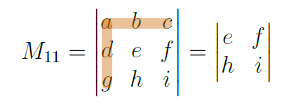
There are new individuals in equation 4.17, the determinants represented by the letter M. Allow me to introduce you to the minors. A minor is the determinant of a square matrix that results from removing some rows and columns from the original matrix. The clue on which row and column to remove is in its index, so, for example, M₁₁ suggests that we should remove the first row and the first column from the original matrix:

M−→DOavirgrinegicittnuidoen

The only elements we haven’t spoken about from equation 4.12 are the pivots, another name I know, but these are just the fellows a, b and c. They happen to all be on the same row. We can generate a new formula for the determinant with all of this information. I have a suggestion, what if we fix a row or a column? Let’s start with a column, and we can define the determinant such that:

∑ 3 det(A ) = (− 1 )i+j a M ij ij j=1

(4.18)

If we set i = 1, we obtain equation 4.17. The question now, is whether equation 4.18 works for n dimensions? And the answer is yes, it does. But, there’s more we can say, as this theorem has a special name, the Laplace expansion:

n ∑ i+j det(A ) = (− 1 ) aijMij j=1

The Laplace expansion works for any row with a fixed column, or for any column if we fix the row. The determinant formula has been broken down, but there is another linear algebra concept we can learn from this, the cofactors. Don’t worry. You have enough knowledge to compute these as they are a part of the formula for the determinant. So, if you multiply (−1)^i+j by the minor M_ij, you will then be computing the cofactor C_ij. The result of this will be a real number because we are multiplying the resultant of a determinant by 1 or -1. In the example above, where we derived the minor M₁₁, the cofactor C₁₁ is equal to:

| | |e f | 1+1 2 || || C11 = (− 1) ⋅ M11 = (− 1 ) ⋅ |h i | | |

Meaning that each entry of a square matrix will have a cofactor, and therefore we can define a matrix of cofactors as:

( ) C11 C21 ⋅⋅⋅ Cn1 | C12 C22 ⋅⋅⋅ Cn2 | | . . . . | Cn ×n = || .. .. .. .. || ( C C ⋅⋅⋅ C ) 1n 1n nn

Ending this with an example will be the best way I feel. So, say that we have G, a 3 × 3 matrix defined as:

( ) 1 4 5 | | G = | 9 2 4 | ( 3 5 10 )

Let’s use the Laplace expansion to compute the determinant. I will select the first row, so j = 1. For my pivots I will have positions g₁₁, g₂₁ and g₃₁ and the signals are +,-,+ respectively. For minors with j = 1 we have M₁₁, M₂₁ and M₃₁. Okay, we have everything we need for this calculation, so let’s get it done:

det(G ) = g11 ⋅ M11 − g21 ⋅ M21 + g31 ⋅ M31

Which is the same as:

| | | | | | |2 4 | |9 4 | |9 2 | || || || || || || det(G ) = 1 ⋅ |5 10| − 4 ⋅|3 10 |+ 5 ⋅|3 15| | | | | | |

The result is

det(G ) = − 117

While I don’t imagine that anyone will be doing a lot of manual computation of the determinant, understanding it is crucial. And if you think that the only use for it is to understand the scale and direction of transformation, you have got another thing coming, as determinants can also be used to invert matrices.

4.2.3 Let’s Go The Other Way Around – Inverse of a Matrix

Would you send a friend from your house to another location without telling this person how to get back? Then why the hell would you do this to a vector? We now know that matrices can represent linear transformations and we also know that this mathematical concept transforms vectors in space. If A is a linear transformation, then, its inverse is also a linear transformation. The difference is that the inverse of A returns the vector back to its initial state. Just as any real number has an inverse, a matrix will also have an inverse, well… OK, I admit not all of them do. In reality, there is a condition that the determinant of such a matrix must meet. If the inverse matrix depends on the determinant, then this same matrix must consequently be a square matrix. There is a particular case for a determinant value that is worth taking a closer look at, namely when the value is 0. If the determinant is a scaling factor, what will it mean if we change the shape by a value of 0? It means that we have lost at least one of the dimensions. In the case of a parallelogram, the result will be a line or a point. An example would be:

( ) 1 1 G = ( 1 1 ) with det (G ) = 1 ⋅ 1 − 1 ⋅ 1 = 0

Consider two vectors −→ g = (3, 1)^T and −→ t = (1, 2)^Tsuch that:

−→−→ xy−123−123tg11

Figure 4.16: The representation of two vectors to aid with the inverse concept

Now let’s calculate the coordinates of the new vectors −→ g∗ and −→ t∗ which are the vectors that result from transforming and by G. This means that −→ ∗ g = (4, 4)^T and −→ ∗ t = (3, 3)^T:

−→−→ xy−1234−1234−→−→gttg∗∗11

Figure 4.17: Showcase of the mappings of −→ g

and

via G.

As expected, the two transformed vectors landed on the same line, and therefore the area of the blue transformed parallelogram is 0.

There is no way to return to the original parallelogram once we arrive on a point or a line, at least with linear transformations. Hence, the second condition for a matrix to have an inverse is that the determinant must not be 0. The last condition is similar to what with real numbers. Consider the inverse of 5. It is defined by x ∈ ℝ such that 5.x = 1, meaning that x = 1 5 . The concept is the same in the case of matrices, but multiplying two matrices won’t result in a scalar. It will result in a special matrix called the identity, represented by I_n. The identity is a matrix in which all elements on the diagonal have a value of 1 and all of the non diagonal elements are 0. The matrix diagonal is formed by all the elements a_ij = 1 where i = j:

Matrix A with a highlighted diagonal

The identity matrix can then be defined as:

( ) 1 0 ⋅⋅⋅ 0 | | | 0 1 ⋅⋅⋅ 0| I = | 0 0 ... 0| |( |) 0 0 ⋅⋅⋅ 1

To arrive at a glorious finish with the hope of prosperity, we still need two more things: a visual way to compute the inverse of a matrix, and a numerical example. Moving on to the visualisations:

xy−−12−12−→−→jj∗211

Figure 4.18: A rotation of −→ j

In the plot, −→ j is (0, 1)^T and its transformation −→∗ j takes values (−1, 0)^T. So, the linear transformation responsible for this (responsibility is terrifying when it’s said out loud, every time somebody asks ‘who’s responsible’ for something, you know something is coming) can be defined as:

( ) 0 − 1 M = ( 1 0 )

What we wish to do now is derive M⁻¹ such that M ⋅ M⁻¹ = I, right? Yes, this is what we defined previously. As this is a simple example, we know that, in order to calculate M⁻¹ we need to define a linear transformation that also does a 90 degree rotation, but in the other direction. So, let’s do it in two steps. Firstly, to rotate a vector 90 degrees clockwise, one needs to place the original y coordinate of the vector in the place of the x coordinate and then place the inverse of the initial x coordinate, −x, in the place of the original y coordinate, such that:

M − 1 : ℝ2 → ℝ2

(m1, m2 ) → (m2, − m1 )

Let’s test this out. If we transform −→∗ j with the linear transformation M⁻¹, we should get the vector −→j such that:

( ) ( ) ( ) 0 1 − 1 0 ( − 1 0) .( 0 ) = ( 1 )

Which is precisely the vector −→ j . So, in theory, if we multiply M by M⁻¹, we need to get I, the identity matrix. Otherwise, something is not right:

( ) ( ) 0 − 1 0 1 − 1 ( ) ( ) M ⋅ M = 1 0 . − 1 0

( ) ( ) 0 ⋅ 0 + (− 1)(− 1 ) 0 ⋅ 1 + 0 ⋅ 0 1 0 = ( 0 ⋅ 1 + (− 1) ⋅ 0 1 ⋅ 1 + 0 ⋅ 0) = ( 0 1)

So far, we have defined a few properties regarding the inverse of a matrix, and I feel that it is a good moment to put them in a little box to produce a summary of where we stand. So, if A is such that A⁻¹ exists, this means that:

A is a square matrix.
A⁻¹ is such that A ⋅ A⁻¹ = I.
The determinant of A is not 0. I will throw another name your way, generosity is the word of the day. When a matrix has this property, it is called non-singular.

The question now is how can we compute an inverse of a matrix? There is a relationship between the determinant of the multiplication of two matrices. We can show that this is equal to the multiplication of the matrix determinants:

det (A ⋅ B ) = det (A ) ⋅ det (B )

(4.19)

If we replace B with the inverse of A:

− 1 det(A ⋅ A ) = det (I) = 1

(4.20)

From equation 4.19 we can write 4.20 as:

det (A ) ⋅ det(A − 1) = 1

It follows then that:

− 1 1 det(A ) = -------- det(A )

Finally we have:

1 A − 1 = --------(adj (A )) det(A )

There is some new information in this formula, I am talking about adj(A). Thankfully, we have enough knowledge to derive this very easily. The adjugate is simply the transpose of the cofactors matrix, C, so we can express this as:

T adj (A ) = C

If you do not recognize the T exponent associated with a matrix, don’t worry, papy is here once more to hold your hand. This means that we will swap the rows with the columns, implying that a matrix with dimensions n × m will become a matrix with dimensions m × n, for example:

( ) 1 4 || 9 5 || A = ( 8 2 )

The transpose of this matrix will still be a matrix, and the notation for it is A^T. The resultant matrix will be:

( ) 1 9 8 T ( ) A = 4 5 2

Given that we have computed the transpose of a matrix for a particular case, let’s derive the general formula, so we can apply it to any matrix or vector of any dimension. A transposed matrix of dimensions n × m is a new matrix of size m × n in which the element in the i_th row and j_th column becomes the element in the i_th column and j_th row:

[ ] AT = [A ] ij ji

Don’t worry, I did not forget the numerical example! Let’s say that the matrix A is defined as:

( ) 1 1 A = ( 0 1 )

Now we need to compute the determinant and the adjugate:

| | ( ) |1 1 | 1 − 1 || || ( ) det(A ) = |0 1 |= 1 and adj (A ) = 0 1 | |

( ) 1 − 1 − 1 1- ( ) A = 1 ⋅ 0 1

Finally it follows that that the inverse of A is:

( ) 1 − 1 − 1 ( ) A = 0 1

The matrix A is known to us. We used it when speaking about a change of basis. The vector that we used at the time was −→ v = (2, 3)^T and the coordinates of −→v in the new basis were (5, 3)^T. So, we must obtain (2, 3)^T if we multiply (5, 3)^T by A⁻¹. We will now be sending this vector back:

( ) ( ) ( ) ( ) 1 − 1 5 1 ⋅ 5 − 1 ⋅ 3 2 ( 0 1 ) ⋅ ( 3 ) = ( 0 ⋅ 5 + 3 ⋅ 1 ) = ( 3)

Bullseye! That is precisely the result we were looking for, so 50 points for us!

This all started with a linear transformation, but we ended up covering a lot of linear algebra concepts that are needed if we are to fully understand these functions. Mastering mappings that promote movement amongst vectors was crucial in my machine learning journey as a data scientist. The graphical component of such a concept allowed me to think about matrices differently, as a vehicle for movement in space. By doing this, ideas like multiplication of a vector by a matrix, matrix to matrix multiplication, determinants, and inverting matrices became explicit, as I had developed a visual concept of what was happening with these notions when they are applied. If you are wondering where to use all of this mathematics in machine learning, well, neural networks are an excellent example to study. And there is yet another case for matrix representation that is worth exploring: systems of linear equations.

4.3 Gatherings in Space – Systems of Linear Equations

First, let’s define a system; and to do that, we will use a vernacular that would impress any executive in an interview room. A system is a collection of components that accepts an input and produces an output. When these systems are linear, we have robust mathematical definitions and concepts that allow us to extract such outcomes, which we can also call solutions. Well, as this book is about linear algebra, this robustness will be provided through methods that we can derive with all of the knowledge we’ve acquired so far. For the components we have linear equations, and for the inputs and outputs we have vectors. A linear system will then be a set of linear equations that receives a vector and produces one, several, or no solutions. For illustration purposes let’s consider a two dimensional scenario as a generic system that we can represent with the following notation:

{ ax1 + bx2 = c dx1 + ex2 = f

(4.21)

In the system 4.21, elements a,b,c,d,e,f are scalars that belong to ℝ and define the system by characterizing two equations which are lines. The solution is defined by x₁ and x₂, which can be unique, nonexistent, or non-unique:

xy−123123xy−123123xy−123123 111

Figure 4.19: The three possible cases for the type of solutions of a system.

The plot above provides a graphical interpretation of some possible type of solutions of a linear system. The blue and yellow lines have for features the scalars a,b,c,d,e,f. If the values are such that the lines are parallel (as shown in the left-hand graph), then the system has no solutions. Conversely, if the lines land on top of each other (as shown in the middle plot), then the system has an infinite number of solutions. Lastly, as seen in the right-hand graph, if the lines intersect each other, this reflects the case where a system has a unique solution. Where are the matrices and the vectors? I miss them too, just like a dolphin misses SeaWorld. But don’t worry, we can represent the system 4.21 with matrix-vector notation:

−→ −→ A ⋅ x = b

The letter A represents a matrix whose elements are the scalars a,b,c,d. The vector −→ x is the solution we are looking for (if it exists). Finally, −→ b is another vector. The best way to define this vector is to look at linear transformations. If A represents a linear transformation, then what we are saying here is that we want to find a vector , that when transformed by A, lands on . So, is where the solution has to land after being transformed by A. Our system can be defined by:

( ) ( ) ( ) a b x1 c ( d e) .( x ) = ( f) 2

If we perform that multiplication, we will end up with the same system of equations 4.21, and the symbol means that we are looking for an interception. However, it is also true that these systems can have as many equations as we wish with as many variables as desired. Consequently, finding a solution for some of them can be portrayed as complicated. Spending a long time doing calculations, only to conclude that there is no solution, is not ideal. Gladly with a matrix representation of such systems, we can understand what is the deal with these so-called solutions, before, doing any calculations towards finding them. We know that for two vectors to intercept somewhere in space, they need to be linearly independent. Therefore, the determinant of a matrix that has these same vectors for columns cannot be zero. From this, it follows that for a system to have a unique solution, the determinant of the matrix that represents the system must be non-zero.

Less talking, more examples, right? Consider a system defined as:

{ − 5x + 2x = − 2 1 2 − 4x1 + x2 = − 4

(4.22)

We now should verify if there is a solution for the system 4.22. For that, we need a matrix A:

( ) − 5 2 A = ( − 4 1 )

The determinant of A is then calculated by:

| | |− 5 2| | | ||− 4 1|| = − 5 ⋅ 1 − 2 ⋅ (− 4 ) = − 5 + 8 = 3 | |

The coast seems to be clear. We have a non-zero determinant, meaning that this system will have a unique solution, and we can proceed to learn how to calculate it. But, before jumping into the deduction of a methodology to find solutions for a system, let’s quickly go over an example where the determinant is zero. Say that B is:

( ) 3 1 B = ( 6 2 )

The determinant of B is equal to zero, det(B) = 3 ⋅ 2 − 6 ⋅ 1 = 0, and visually:

−→−→ xy−12345−123456bb1211

Figure 4.20: Linearly dependent vectors due to a zero value determinant.

As expected, those vectors are linearly dependent. The angle formed by them is 0 degrees. Okay, but the system 4.22 has to have a solution because the determinant of A is not 0. To find it, let’s get the vector −→ x represented by:

( ) −→ x1 x = ( x2 )

The only thing missing is the vector −→ b . Now, is not as badass as −→ x because, can take any value for coordinates. On the other hand, has fewer options, much like a politician:

( ) − 2 −→ b = ( − 4)

The equation below represents the system in question:

−→ A −→x b ◜( ---◞◟--)-◝ ◜( -◞◟)-◝ ◜( -◞ ◟)-◝ − 5 2 x1 − 2 ( ) ( ) ( ) − 4 1 ⋅ x2 = − 4

Let’s pause for a moment to observe the representation above, that is if you don’t mind. A is a matrix that represents a linear transformation, and −→ x is a vector. We know that A. will map into a new vector. The restriction now is that the resultant recast vector of that transformation has to be equal to another vector, −→ b :

−→−→−→−→−→ xy−−−−−12345−−−−12345jijb−→xi∗∗654325432

Figure 4.21: The graphical representation of a system of linear equations.

The plot is populated, but let’s take it step-by-step. The vectors −→ i and −→ j represent the standard basis. A generic vector is represented by −→ x , so please ignore the coordinates (2, 4). It is just for a visual representation. Now, −→ ∗ i and −→ ∗ j are the new basis as they are the result of the transformation of A on −→ i and −→ j . The vector −→ b is where we need −→x to land. There are several ways to get the solution for that system, we will focus our attention on a technique called the Cramer’s rule. As while it may not be the most efficient approach, it is the method with the best visual component. In this case, best means efficient in terms of computation. Our goal is not to learn how to calculate these solutions by hand. We have computers to do that. Instead, we just want to understand what is happening so we can better analyse the results.

Let’s start by grabbing three elements from the plot above: the basis formed by the vectors −→ i and −→ j , and the generic vector −→ x . Consider the following plot:

−→−→−→ xy−123−123xijx211

Figure 4.22: The first plot of Cramer’s rule.

The vector −→ x represents any vector that verifies a system of equations; its coordinates are (x₁,x₂). In this case, the blue parallelogram has an area equal to 1.x₂, meaning that the value of this area is equal to x₂. Let’s be rigorous here; it is not the area, but rather the signed area, because x₂ can be negative. We can make a similar case with the other coordinate in −→x , a parallelogram with an area of x₁ instead of x₂:

−→−→ xy−23−123ij−→xx111

Figure 4.23: The second plot of Cramer’s rule.

The signed area of the blue parallelogram will be 1.x₁, resulting in x₁. These parallelograms can also be built with the transformed versions of −→ i , −→ j and −→x . Let’s start with the vector −→ i∗ that has coordinates (−5,−4). But instead of −→x , we have −→ b , which is the result of transforming −→ x with A:

−→−→ xy−−−−−−1−−−−−−1i∗b 765432765432

Figure 4.24: The solution of the linear system.

In the plots 4.22 and 4.23, we drew two different parallelograms. One with the vector −→ x and −→ i , and the other formed by and −→ j . These have areas values of x₂ and x₁ respectively. Following this, we transformed and to obtain a new parallelogram which we don’t yet know the area of (as shown in the figure above). In order to derive x₂, one must find some relationship between the areas of the original and transformed parallelograms. Fortunately, we have a scalar that provides information relating to the magnitudes by which sizes are scaled via linear functions. So, if the area of the original parallelogram was x₂, this new shape will have an area of det(A) ⋅ x₂:

Area = det (A ) ⋅ x 2

-Area--- x2 = det(A )

We know the coordinates of vector −→ b and we know where it lands, so we can create a new matrix:

( ) − 5 − 2 ( − 4 − 4)

The determinant of this matrix will represent the area of the transformed parallelogram:

|| || |− 5 − 2| ||− 4 − 4|| | | x = -|------|--= (−--5)-⋅ (−-4)-−-(−-2)-⋅ (−-4) = 12- = 4 2 |− 5 2| (− 5) ⋅ 1 − 2 ⋅ (− 4 ) 3 || || |− 4 1| | |

If we want to derive a formula to compute x₁ it is done in the same way as was shown for x₂. The only difference is that we will transform the vector −→ j and use its transformed version alongside −→ b to build the new parallelogram:

Area = det (A ) ⋅ x1

Area x1 = -------- det(A )

We know the coordinates of vector −→ b , so:

| | ||− 2 2|| |− 4 1| | | |-------| (−-2-) ⋅-1-−-(−-2-) ⋅-(−-4) 6- x1 = || || = = = 2 |− 5 2| 3 3 |− 4 1| || ||

We have found that the solution for our system is the vector −→ x = (2, 4)^T. Indeed there are computers that can tally all of these tedious calculations, almost like having slaves without any feelings. I wonder what will happen if they ever get to the point of sentience. Will they miraculously channel all of their pain into the creation of new styles of dance and music that we can enjoy, even after the way we have treated them? Or will it be judgement day, and someone, John Connor style, will have to save us? I hope I haven’t lost you because you’re too young to have seen The Terminator? All the same, this technique is here to help you visualise what is happening. And, if you do choose to use a computer to solve a system, you won’t think that these black boxes are performing magic. Also, this showcases a situation that often occurs in mathematics, in which there are several ways to solve the same problem. The task was to find a new vector that, when transformed, would land on a specific set of coordinates. The method for finding a solution was derived based on areas. Another way to solve a linear system is Gaussian elimination, which won’t be covered here, though if you wish to learn it, I will say that you will have no problems with it. There are still two things missing: we need the general formula for Cramer’s rule, and we should verify what happens when we transform the vector −→ x with the linear transformation A. First things first, Cramer’s rule. Consider a linear system represented as follows:

−→ A −→x = b

Where A is a squared matrix with size n × n, −→ x = (x₁,x₂,…,x_n)^T and −→ b = (b₁,b₂,…,b_n). We can then define the values of the vector by:

det (A ) xi = -------i- det(A )

The value det(A_i) is the matrix formed by replacing the i_th column of A with the column vector −→ b . Next, for the verification part, we have to transform (2, 4)^T with A and to check if we get :

( ) ( ) − 5 2 2 ( − 4 1 ) ⋅( 4)

( ) ( ) − 10 + 8 − 2 ( ) ( ) = − 8 + 4 = − 4

Linear systems have many applications, but for now, I would like to explore four particular types of systems with some important characteristics. Consider a matrix A_m×n that maps vectors from ℝⁿ to vectors in ℝ^m. Let’s also define two vectors, −→ x and −→ y . The different systems that are worth paying special attention to are:

A ⋅≠0 row space of A.
A ⋅ = 0 nullspace of A.
A^T ⋅≠0 column space of A.
A^T ⋅ = 0 left nullspace of A.

The equations above define important subspaces in the field of linear algebra. A subspace is a space within another vector space where all the rules and definitions of vector spaces still apply. In case one, we are performing row-wise dot products with a vector −→ x , and our interest lies in the calculations performed between rows that are not perpendicular, so that the result is not zero. This subspace is called the row space. On the other hand, in equation number two, we want a subspace where every vector is transformed to zero. This is called the nullspace. Finally, cases three and four represent very similar concepts, but as we are now computing dot products with the transpose of A, these subspaces are for the columns instead of the rows. So, case three is the row space, while case four is the left nullspace. There must be a relationship between the dimension of the space spanned by A and the subspaces that are part of A, namely those defined by the four systems shown above. To understand these relationships, we need to introduce another concept: rank. The rank of a matrix is the dimension of the vector space generated by its columns, meaning that it is also the basis of the column’s space. Let’s consider a matrix A_4×3 defined as:

( ) 1 2 0 | 1 2 1 | || || A = | 2 4 − 1| ( 3 6 0 )

To calculate the rank of A, we need to understand how many linearly independent columns exist in matrix A. This quantity will also give the number that defines the dimension of the column space. After a closer look, we can identify that the first column is half of the second, and there is no way of getting the third column by combining the first two, or by scaling any of them. So the matrix has a rank equal to two. There are two linearly independent vectors, (1, 1, 2, 3) and (0, 1,−1, 0), and they form a basis for the column space. Now, let’s compute the nullspace of A. This space is such that {x ∈ ℝ³ : A. −→ x = −→ 0 }. We are looking for all of the values of in ℝ³, when transformed by A, result in the null vector, which is equivalent to:

( 1 2 0 ) ( ) ( ) x1 0 || 1 2 1 || | | | | | 2 4 − 1| ⋅| x2| = | 0| | | ( x3) ( 0) ( 3 6 0 )

So it follows that:

( || x1 + 2x2 = 0 ( || | x1 = − 2x2 { x1 + 2x2 + x3 = 0 { ⇔ x3 = 0 ||| 2x1 + 4x2 − x3 = 0 |( |( 3x1 + 6x2 = 0

I am about to drop some more notation so brace yourselves. The nullspace is represented by:

nullspace (A ) = { (c,− 2c, 0) : c ∈ ℝ }

And in this particular case, it can also be represented by:

Span {(1, − 2, 0)}

The dimension of the nullspace, which is also called the nullity(A), is equal to one, meaning that the basis of that space has only one vector. At this point, we have the dimensions of the column space and the nullspace: two and one respectively. Coincidentally or not, the dimension of the column space, which is equivalent to the rank of A plus the dimension of the nullspace, is equal to the number of columns in A. Obviously this is not a coincidence at all; the theorem of rank-nullity states that:

rank + nullity (A ) = n

(4.23)

The proof of this theorem is extensive, and I will omit it, but what we can take from it will be extremely useful. The rank of A plus its nullity equals n, the number of columns. Apologies, but we must introduce another simple definition at this time, for the term full rank. A matrix A of size m × n is said to be of full rank when the rank is equal to the min(m,n). There are two possibilities to consider: m ≥ n and m < n. But why would we care about this? Well, it just so happens that we can understand the dimension of the nullspace when a matrix is of full rank by just looking at the order of magnitude of m and n. If A is of full rank and m < n, the rank of A is equal to m. By equation 4.23, we have m + nullity(A) = n, which is the same as:

nullity (A ) = n − m when m < n and A is full rank.

On the other hand, if m ≥ n, it follows that the rank of A is equal to n, so the nullspace has a dimension of 0:

nullity (A ) = n − n = 0 when m ≥ n and A is full rank.

If the matrix is square, then n = m, so it makes sense that a square matrix is of full rank when the rank of A is equal to n. There are a couple more relationships between the nullity, the rank, and the determinant that are worth studying. Let A be such that:

( ) A = −→v −→v ... −→v 1 2 n

Where all the vectors −→ v are the columns of A. With this, the equation for nullity can be expressed by:

( ) ( ) x1 0 ( ) | | | | A. −→x = −→0 ⇔ −→ −→ −→ ⋅ | x2 | = | 0 | v1 v2 ... vn ( ... ) ( ...) xn 0

Which is the same as:

−→ −→ −→ −→ x1 ⋅ v1 + x2 ⋅ v2 + ...+ xn ⋅ vn = 0

(4.24)

If we say that all the vectors are linearly independent, the only way for equation 4.24 to be verified is for all of the factors represented by the x’s to be equal to 0. Otherwise, it will be possible to get at least one term as a function of another; consequently, the assumption of linear independence won’t be valid. Therefore, if the nullspace is of dimension zero, it also means that the determinant is non-zero. As you can see, the rank provides a lot of information about linear transformations and is an excellent way of exploring some of their characteristics.

When introducing the rank and deducing its relationships and properties, we paid a lot of attention to the nullspace of a matrix. This space is also essential when it comes to introducing one more notion, the last one before we vault into the concepts that are often used in machine learning: the principal component analysis and the single value decomposition.

Even though we are already well-equipped in terms of linear algebra knowledge, the feeling in the air is that everything really starts here. Let’s initiate this new part of the odyssey by defining a particular case of a linear system. What if we wish to find a vector −→ v that, when transformed by A, lands on or on a scaled version of it? Before, we were looking for a vector −→ x that, when transformed, would land on a generic vector −→ b . We can define a scaling factor by λ and formulate the system with the following equation:

−→ −→ A v = λ v

(4.25)

4.3.1 Line Up Vectors! The Eigen Stuff

Good people of the sun, allow me to introduce you to the Eigen ”stuff”. These vectors −→ v that, when transformed by a matrix, land on itself or on a scaled version of itself are called the eigenvectors. They happen to be like the police as they are always with someone else, so for each eigenvector, you will have a corresponding eigenvalue λ, the scalar by which the vector stretches or shrinks. To put it simply, think of a matrix as a machine that rotates and/or scales vectors. An eigenvector is a vector that, when put through this machine, only gets stretched or shrunk by a certain amount but does not get rotated:

−→−→−→−→−→∗∗ xy−−−−12−−−−12ijijv 54325432

Figure 4.25: A reminder of the representation of a linear system.

In the plot above, −→ i∗ , −→ j∗ represent the transformed version of the standard basis , . We are looking for one or more vectors that, when modified by A, land on a linear combination of −→ v :

−→−→−→−→ xy−−−1234−−−1234vvvv123432432

Figure 4.26: A mosh pit of vectors: some possibilities for eigenvectors.

We have a few examples of eigenvectors in the plot above, and, as they are all linear combinations of each other, they all land on the black line that represents that particular vector span. Let’s manipulate equation 4.25 to get it into a format where the computation of both the eigenvectors and eigenvalues will be more straightforward. It is hard to find a good use case for manipulation. However, perpetrating this act to produce an equation still seems to be accepted. So far, nobody seems to care, and it comes with benefits for the mathematician. Let’s exploit this:

−→ −→ A v = λ v

We’ve learned about the identity matrix on our journey into linear algebra, and so we can say:

−→ −→ A v = λI v

Multiplying the identity matrix I by a given vector −→v will result in the vector −→ v . That equation is equivalent to:

−→ −→ −→ A v − λI v = 0

We can then write it as:

(A − λI )−→v = −→0

(4.26)

There are two ways for 4.26 to be verified. The first one is not very interesting (the trivial solution). This is when −→v = 0. That told us nothing, so we need to find a −→ v other then = 0. The element (A−λI) is a matrix whose diagonal elements are part of the diagonal of A minus the scalar λ, something like:

( ) ( ) ( ) a b λ 0 a − λ b ( ) ( ) ( ) c d − 0 λ = c d − λ

So, equation 4.26 can be depicted as:

( ) a − λ b ( c d − λ) ⋅−→v = 0 ◟ -------◝◜--------◞ R

(4.27)

Ideally, we would have an equation where we can apply some technique and calculate the λ′s. If you recall, the determinant is a function that takes in a matrix and spits out a scalar, and we have a formula for it, so this might be an excellent path to follow to find an equation where we can isolate λ. However, the determinant alone won’t be enough to get us to where we need to be. That zero on the right side of the equation causes constraints, and we need to consider them. Thankfully, there is a way to create a relationship between the determinant and zero. For example, consider the inverse of a matrix. For a matrix to have an inverse, its determinant has to be non-zero. In addition, it comes to mind that, if a matrix is invertible, the multiplication of this given matrix with its inverse results in the Identity matrix. Maybe we can work with this. Let’s define the inverse of R by R⁻¹ and replace this notation with 4.27:

R − 1 ⋅ R ⋅ −→v = R − 1 ⋅ −→0

This results in:

−→ I ⋅ −→v = 0

And that is as valuable as an ashtray on a motorbike. We specifically stated that −→v = 0 was not of interest. But everything’s not lost. What follows is that R must not be invertible, and like that, we guarantee any non-trivial solution! So, if R has no inverse, the determinant of that specimen must be zero:

det (A − λI ) = 0

Geometrically, this also makes sense. We are transforming a vector −→ v into a linear combination of itself. For that, the determinant has to be zero, as we saw previously. Let’s follow an example and use A as the linear transformation:

|( ) ( ) | | − 5 2 λ 0 | ||( ) ( ) || | − 4 1 − 0 λ | = 0 | |

This is equivalent to:

| | |− 5 − λ 2 | || || | − 4 1 − λ| = 0 | |

(− 5 − λ )(1 − λ) − 2 ⋅ (− 4 ) = 0

λ2 + 4 λ + 3 = 0

From our fundamental maths knowledge we know that the roots for that equation can be calculated with the following formula:

√ ---------- −-b-±----b2-−-4ac-- x = 2a

Where:

2 ax + bx + c = 0

Okay, so applying that formula to our equation gives us the following values for λ:

λ = − 3 and λ = − 1

We now have the scaling values that will stretch or squish the eigenvectors, but we still do not have the vectors. However, there is a formula that allows us to get these vectors: 4.26:

−→ (A − λI )−→v = 0

Given that we know the λ values, we can compute the eigenvectors. Let’s try with λ = −3.

( ) ( ) − 5 − (− 3) 2 v1 ( ) ( ) −→ − 4 1 − (− 3 ) ⋅ v2 = 0

( ) ( ) − 2 2 v1 ( ) ( ) −→ − 4 4 ⋅ v2 = 0

Let’s name that guy. Should we go for Francis? Maybe it is too much, but M should be enough:

( − 2 2) M = ( − 4 4)

This represents a linear system, but the determinant of the matrix M is zero. Does this make sense? A determinant of 0? This means that we either have no solutions, or a lot of them. The latter is happening here. The coordinate values that verify that the system can be represented by vectors that land on the span of the vector that we are after. There is an implication to this determinant value; Cramer’s rule will be doing a prophylactic isolation and can’t show up. The system becomes:

{ − 2v + 2v = 0 1 2 − 4v1 + 4v2 = 0

This is a simple system that is here as a showcase, therefore we can solve it with a ”maneuver” like this:

{ { − 2v1 + 2v2 = 0 − 2v1 = − 2v2 ⇔ − 4v1 + 4v2 = 0 − 4v1 + 4v2 = 0

{ { v = v v = 1 1 2 ⇔ 1 − 4v1 + 4v2 = 0 v2 = 1

So, the eigenvector corresponding to the eigenvalue λ = −3 is the vector (1, 1)^T, let’s call it −→ t :

xy−−12−−12−→t2121

Figure 4.27: The first eigenvector of the example.

If we transform −→ t with A, −→ t∗ , the transformed version of needs to land on that black line. It has to be the vector (−3,−3)^T; let’s verify this:

( ) ( ) ( ) − 5 2 − 1 − 3 ( − 4 1 ) ⋅( − 1) = ( − 3)

xy−−−123−−−123−→t−→t∗321321

Figure 4.28: The transformation of a eigenvector.

Okay, that verifies the calculations. If we do something similar to that with λ = −3, but now with the other eigenvalue, λ = −1, we end up with:

( ) ( ) − 5 − (− 1) 2 v1 ( ) ( ) −→ − 4 1 − (− 1 ) ⋅ v2 = 0

( ) ( ) − 4 2 v1 −→ ( − 4 2) .( v2 ) = 0

I will omit some of the steps of the calculations as they are like the ones that we did for the other eigenvalue, but this time, the eigenvector is equal to −→v = ( 1 2 , 1)^T. Similarly, if we transform −→v into −→v ∗ making use of the linear transformation A, −→ ∗ v has to land on the same line as −→ v . Let’s verify:

( ) ( 1) ( 1) − 5 2 2 − 2 ( − 4 1) .( 1 ) = ( − 1 )

As expected, the resultant vector is a linear combination of the original vector that we transformed with the matrix A. Let’s visualise this result:

−→−→ xy−−123−−123vv∗3232

Figure 4.29: The second transformation of an eigenvector.

In essence, we found a particular group of vectors that, when transformed, land on its span. If you are doubtful about the utility of this concept, I empathise with that, but allow me to try to convince you that this was not an attempt to put a few more pages in this book so that it gets to at least 100 pages! So, let’s bring back the 90’s! Sorry, I mean matrix A, its eigenvalues, and the respective eigenvectors:

( ) ( ) − 5 2 −→ 1 A = ( − 4 1) , λ = − 3, t = ( 1)

( 1) 2 λ = − 1, and −→v = ( 1)

As a friendly reminder, this is how we can represent the system to calculate the eigenvalues:

−→ −→ A v = λ v

Okay, if we now replace −→ v and λ with each eigenvalue and eigenvector pair, we can form two different equations:

( ) ( ) 1 1 ( ) ( ) A 1 = − 3 1 ( 1 ) ( 1) 2 2 A ( 1 ) = − 1 ( 1)

(4.28)

So, we have two vector equations. By forming one matrix with the eigenvectors and another with the eigenvalues, we can combine the two equations in 4.28 into a single equation with matrices:

◜ --P◞◟---◝ ◜--P◞◟---◝◜ ----◞Λ◟-----◝ ( 1) ( 1 ) ( ) 1 2 1 2 − 3 0 A ( 1 1) = ( 1 1 ) ( 0 − 1 )

Algebraically we have:

AP = P Λ

(4.29)

When we studied the inverse of a matrix, we concluded that for a matrix A⁻¹ to be the inverse of A, AA⁻¹ = I. So, if we want to isolate A on the left side of equation 4.29, we can multiply both sides of the equation by P⁻¹:

AP P − 1 = P ΛP − 1

Which becomes:

− 1 A = P ΛP

(4.30)

4.3.2 I’ve Got the Power, to Power – Matrix Diagonalization

So, we can define A as a product of three other matrices, including the eigen base P and its inverse P⁻¹ which represent two rotations. On the other hand, the matrix Λ is a diagonal matrix with eigenvalues for elements. On this matrix are the scaling terms of equation 4.30. So, what’s happening here is that we are representing a matrix by two rotations and one scaling term. Since we have a linear transformation that is split into three different matrices, it is worth taking a look at the properties of these matrices.

One of them stands out: Λ, which is a diagonal matrix. The only time we dealt with a matrix of this type was when the identity I was involved in our calculations. It turns out that this class of matrices, the diagonal ones, has some pretty incredible properties that make operations much lighter and more manageable. For example, to calculate the determinant of a matrix with this form, one only needs to multiply the elements that form the diagonal. Let’s consider A to be a diagonal matrix defined as:

( ) a 0 ( ) A = 0 b

By definition, the determinant of A is:

|| || |a 0 | ||0 b ||= a ⋅ b − 0 ⋅ 0 = a ⋅ b | |

A has two dimensions, and these are always simple cases. However, if we have matrices of higher dimensionality, the calculations for the determinant are now more straightforward than the ones for non-diagonal matrices. Let’s now consider a matrix A with three dimensions:

( ) a 0 0 | | A = | 0 b 0| ( 0 0 c)

We know that we can pick a row or a column and apply the Laplace expansion that we previously defined to calculate the determinant. If you don’t remember, there is no need to feel bad or even go look for it. Here it is again:

∑ n det(A ) = (− 1 )i+j a M ij ij i=1

As you can see, in this formula, an element of the matrix is multiplied by a minor, a_ij. As this is a diagonal matrix, the only non-zero elements are those on the diagonal when j = i, so the determinant will simply be:

2i det(A ) = (− 1 ) aiiMii

This is the same as multiplying all of the elements on the diagonal together. It is fair to assume that if we can simplify the calculation of the determinant for a diagonal matrix, then the computation of its inverse will also have a more straightforward formula, and it does! Previously we specified that:

1 A − 1 = -------(adj (A )) det (a)

If we have all the 0 entries excluding the diagonal, the matrix adj(A), is equal to:

( ) M11 0 0 | 0 M 0 | adj(A ) = | 22 | ( 0 0 M33 )

This is equivalent to:

( ) bc 0 0 | | adj (A ) = | 0 ac 0 | ( 0 0 ab )

And if we divide that adj(A) by the determinant:

( ) bc 0 0 | 0 ac 0 | |( |) 0 0 ab − 1 A = ----------------- abc

This results in:

( 1- ) a 0 0 − 1 || 0 1b 0 || A = ( 1 ) 0 0 c

This simplifies the calculation of an inverse. So, we have to replace each non-zero element with its inverse. The last thing to mention about diagonal matrices relates to a scenario in which we want to compute multiplications. Let’s define a generic 2 × 2 matrix X as:

( ) x11 x12 X = ( x21 x22)

There are two different scenarios here: The first, matrix multiplication, is not commutative; however, if one of the matrices in the operation is diagonal, we can easily get the results. If X is multiplied by a diagonal on the left, it will change the matrix row-wise. Otherwise, if we are multiplying X by a diagonal matrix on the right, then this will have an impact column-wise. This will apply to any matrix size.

( ) ( ) ( ) x11 x12 a 0 ax11 bx12 ( x21 x22) ⋅ ( 0 b) = ( ax21 bx22 )

( ) ( ) ( ) a 0 x11 x12 ax11 ax12 ( ) ( ) ( ) 0 b ⋅ x21 x22 = bx21 bx22

Secondly, and this will be the most potent fact about this diagonalization technique, we can simplify the multiplication between matrices. As the non-zero elements are all on the diagonal, powering these matrices comes with comfort, as it will only be necessary to power each component of the diagonal. Just to explain, when we say powering, we’re referring to the process of multiplying a matrix by itself, which is the same as raising it by a power.

Okay, the reality is that two-by-two matrices are baby talk. They make clear-cut examples, but when do we have the opportunity to work with only two dimensions in the real world? If you wish to go on with machine learning, you will most likely encounter some big ass matrices, and on top of that, consider the fact that you have to power them with a large exponent. Diagonalization will then come in handy to save the day and the computation bill! We know that A can be represented by:

− 1 A = P ΛP

Say that A is a n × n matrix where n is giant (no joke). Think of a matrix with information about the weather, like states of observable climate conditions, where the matrix entries are probabilities of moving from one state to another. You could model this with some type of sequential model where the states are the weather conditions on a given day. An example of this type of model is a Markov Chain (which we won’t go into right now, but it will be covered on a different book). Under these conditions, there is a case for powering a matrix because it will allow you to understand the system at a given state. So, powering A to the t (where t is large) can be computed by multiplying A by itself t times, which is extremely expensive in terms of computation time . Imagine all the dot products that we’d have to do. But don’t worry, we can make use of matrix diagonalization: instead of…

At = A.A.A...A t times

…we could try and do something different. Let’s start by squaring A:

2 − 1 − 1 A = P ΛP P ΛP

(4.31)

A was replaced by its diagonalization form, and we can simplify equation 4.31, as we know that P ⋅ P⁻¹ is equal to the identity I:

A2 = P Λ ΛP − 1

The matrix Λ is diagonal, so it follows that Λ.Λ is equal to Λ² and the equation becomes:

A2 = P Λ2P − 1

Right, this seems simpler to compute. Let’s check what we can do if we have A³. Well, A³ = A².A, which can be written thus:

3 2 − 1 − 1 A = P Λ P ⋅ P ΛP

Following the same logic as before:

A3 = P Λ3P − 1

Let’s check for A⁴… I am joking, but you see where this is going. If you want to power A to t, the formula is:

t t − 1 A = P Λ P

Powering matrices is a common practice in machine learning. You probably won’t have to write code for it. But still, I can assure you that when you are applying algorithms to data, it is likely that at some point, it will happen. Suppose we try to interpret the equation for diagonalization geometrically. In that case, we see that we can represent a linear transformation as one rotation, followed by a stretch, and then another rotation. Let’s experiment: For that we’ll need a volunteer, anyone? Anyone at all? Mr. −→ u , welcome back, sir. Firstly we will transform it with A. Following this, we will take a longer route, going from P⁻¹ to Λ, and finally to P. Okay, has the coordinates (1, 3)^T, and when mapped by A it results in:

( ) ( ) ( ) − 5 2 1 1 A ⋅ −→u = ( − 4 1) ⋅( 3) = ( − 1)

The plot bellow illustrates the transformation A on −→ u , which we represent with −→ ∗ u :

xy−−−123−−−123−→−→uu321321∗

Figure 4.30: Matrix diagonalization – Where −→ v

needs to go.

Let’s now check what happens if we rotate, stretch and rotate again the vector −→u with PΛP⁻¹. The result has to be a vector with coordinates (1,−1)^T. There is one thing missing. Well, it is more like three; the dam matrices. We have calculated the eigenvectors of A, so we are good in regards to P. It is a matrix with the eigenvectors of A for columns. Now Λ is even more accessible. It is a matrix whose diagonal has for entries the eigenvalues of A, and the remaining entries are 0. That fellow P⁻¹ is the inverse of P, and we already know how to invert a matrix, so we are in no danger of being stuck. With this, we are ready to start, so bring on the first rotation, please, maestro:

( ) ( ) ( ) −→ 2 − 1 1 − 1 −→ P − 1 ⋅ u = ( − 2 2 ) .( 3) = ( 4 ) = u ∗1

Now, let’s scale it:

( ) ( ) ( ) − 3 0 − 1 3 −→ ∗ ( ) ( ) ( ) −→∗ Λ ⋅u 1 = 0 − 1 . 4 = − 4 = u2

Finally, let’s rotate it again:

( 1) ( ) ( ) −→ 1 2 3 1 −→ P ⋅u ∗2 = ( 1 1 ) ⋅( − 4) = ( − 1) = u ∗3

When we rotate −→ u with P⁻¹ we end up with a transformed vector −→ ∗ u 1 that is then stretched by λ into a new vector called −→ ∗ u2 . This is then rotated by P to result in −→ ∗ u 3 which in turn, has the same coordinates as −→u . There is another name for this diagonalization technique. It is also known as eigendecomposition, which is a special case of matrix decomposition:

−→−→−→ xy−−−−−2345−−−−−345−→uuuu5432154321∗1∗2∗3

Figure 4.31: Matrix diagonalization – The full journey of −→v

The only catch is that the matrix that we decompose has to be square. Otherwise, we can’t use this technique. Unfortunately, square matrices are as standard as tax rebates, which means they rarely come by, and, if you do come across one, it is likely you messed up somewhere. Don’t worry, it happens. So, if square matrices are not that common, there’s got to be a way to decompose any matrix shape. And there is. You can refer to it as the single value decomposition, or by its street name, SVD. These techniques of splitting a matrix into a multiplication of newly created matrices with particular characteristics have great visual interpretations. When it comes to introducing this new form for decomposing a matrix, we will focus on that.