The primary objective of this chapter is to inform you about sustainability best practices, along with model governance techniques, to align them with your organizational goals and initiatives. You will be made aware of the environmental consequences of training Deep Learning (DL) models and possible remediating actions that you could take. You will also become accustomed to different metrics of sustainability for different platforms, which will lead to sustainable model training and deployment.

By the end of this chapter, you will have been equipped with the collaborative and decentralized learning techniques involved in Federated Learning (FL), whether model training happens on the network, at the edge, or in the cloud. Finally, you will also be aware of the tools that can help to track carbon emission statistics.

In this chapter, these topics will be covered in the following sections:

• The key to sustainable enterprise-grade AI platforms
• Sustainability practices and metrics across different cloud platforms
• Carbon emission trackers
• Adopting sustainable model training and deployment with FL

This chapter requires you to have Python 3.8, along with some Python packages, listed as follows:

• Keras 2.7.0 and TensorFlow 2.7.0
• pip install CodeCarbon

Sustainability has a very important role to play in the era of ethical AI, as the ability to predict energy emissions can support initiatives to protect the environment and conserve resources. AI-enabled platforms can facilitate emission reductions and carbon dioxide (CO2) removal, which can foster greener transportation networks, as well as monitor and control deforestation. Thus, by effectively using AI solutions in a sustainable manner, we can try to prevent extreme weather conditions.

As a first step, we should understand why organizations have set up a vision to go carbon free. Along with this, it is equally important to understand the leadership vision to properly align teams with the sustainable mission goals set forth by their senior leadership and CXOs.

Hence, as the first step, we will look at the motivation of organizations to restructure their roadmaps toward building sustainable AI solutions.

Sustainable solutions with AI as an organizational roadmap

We should be extremely careful to build solutions that are environmentally friendly. Substantial research indicates that just 40 days of research training can emit 96 tons of CO2. The amount is so large that it can be compared to 1,000 hours of air travel, roughly equivalent to the carbon footprint of 23 American homes (https://www.analyticsinsight.net/new-mit-neural-network-architecture-may-reduce-carbon-footprint-ai/, https://inhabitat.com/mit-moves-toward-greener-more-sustainable-artificial-intelligence/). The carbon emissions involved in running a neural network search have been as high as 600,000 CO2e (lbs), equivalent to the lifetime of 5 cars. Training algorithms such as large Natural Language Processing (NLP) models (or transformers) generate so much energy that data scientists need to be careful when designing the architectures of this kind of DL neural network (https://aclanthology.org/P19-1355.pdf). This kind of training can be threatening to the environment. If we continue to build these AI solutions in this way, future generations will face adverse environmental consequences.

Organizations that want to apply AI to sustainability should not only focus on sustainable banking, energy consumption, or healthcare but also develop best practices to quantify the CO2e by measuring carbon footprints and the computational power required to train and evaluate the methods for managing data centers efficiently.

In addition, data scientists and engineers should first evaluate the need for DL models before choosing them. For certain use cases, similar performance can be guaranteed with a standard model without needing to train a DL model. So, correct practices and audits need to be established in an organization before training DL models, to avoid a large carbon footprint.

Once the data science team finalizes the model (traditional versus DL in either centralized or FL setups), the selection of the number of hyperparameters and careful tuning play important roles in carbon emissions. Tuning hyperparameters for FL can become expensive in terms of energy consumed, as this leads to tuning hundreds of different models (with local models in the clients).

The tuning process in FL may become increasingly complex due to parameterization in the aggregation strategy, as well as heterogeneity in the individual datasets of the clients. The complexity of hyperparameter tuning in both types of learning must be carefully designed to minimize CO2e release.

The team should be aware of the choice of the dataset and the extent of preprocessing and feature engineering involved. One such example is when feature engineering techniques become more exhaustive and expensive in developing recommender systems using financial and retail data rather than using only retail data.

Let us study the organizational standards that can enable the building of such frameworks.

Organizational standards for sustainable frameworks

CXOs and leadership must also be involved in mandating sustainable data and model practices as organizational objectives. These sustainable practices for scalable cloud platforms originate from setting the right objectives and Service-Level Agreements (SLAs) based on the current business requirements. This may require selecting the right trade-off to affect sustainability metrics by prioritizing business-critical functions and allowing lower service levels for non-critical functions. Critically, businesses should handle siloed data across departments by defining architectural design patterns that are suitable for sustainable model training and deployment.

Now, let us begin looking into the metrics measured across different cloud platforms.

In this section, we will explore how we can evaluate the following:

• Useful emission metrics on Google Cloud
• Best practices and strategies for carbon-free energy
• The energy efficiency of data centers

First of all, we will discuss some of the metrics of Google Cloud and also cite some of the initiatives and tools promoted by Microsoft.

Google’s role in sustainable cloud solutions has been overwhelming, and it has been the leading cloud provider in terms of purchasing sufficient renewable energy, more than any other organization. Starting with a pledge in 2007 to become the first major carbon-neutral company by 2017, 100% of its electricity consumption now comes from renewable energy. In the absence of enough wind and solar power or renewable resources, Google draws power from the local grid to run operations at a local data center. Conversely, when sufficient power is available, the excess is fed back to the local grid to be used elsewhere. With a vision of 24/7 carbon-free energy by 2030, it uses the guidelines mentioned in the following sections to make its data centers and electricity grids carbon free.

Microsoft also has its own Power BI application for Azure, popularly known as the Microsoft Sustainability Calculator, which provides insights into the amount of carbon emissions associated with the data centers in each region. Even initiatives such as the purchase of carbon-neutral renewable energy help to drive its annual cloud consumption.

Emission metrics on Google Cloud

To move to carbon-free energy by 2030, Google Cloud has come up with an initiative to empower its customers to leverage carbon-free energy 24/7. Customers can consider the carbon impact when designing their solutions by analyzing a metric called CFE%. This metric quantifies the amount of energy consumed every hour that is carbon free by broadly dividing it into two main categories: CFE% and carbon intensity. CFE% is calculated based on the generated energy that feeds the grid at any time, along with the clean energy attributions (through the supply of renewable energy resources) made available by Google that are applied to the grid:

• Google CFE%: This provides a measure of the average percentage of carbon-free energy. This measure, when computed per location on an hourly basis, provides customers with an estimate of the amount of time that their apps can run on carbon-free energy, depending on the investments made into carbon-free energy that apply to the grid at the same location.
• Grid carbon intensity (gCO2eq/kWh): This metric quantifies the average life cycle of gross emissions per unit of energy from a grid at a specific location. With it, we can compare the carbon intensity of the electricity at different locations within a local grid that behave similarly. Using this, we can select the region of deployment of production apps when two or more locations demonstrate a similar CFE%. To cite an example, we will often see that Frankfurt and the Netherlands exhibit similar CFE% scores, while the Netherlands experiences higher rates of emissions.

Now, let’s discuss the best practices involved in utilizing carbon-free energy.

Best practices and strategies for carbon-free energy

As Google Cloud Platform actively concentrates on increasing the CFE% for each of the Google Cloud regions, a higher percentage of carbon-free energy increases the sustainability of deployments. Some of the unique propositions for cloud AI specialists and architects are as follows:

• Selecting a lower-carbon region: Building and running new applications in low-carbon regions (such as Finland or Sweden) with a higher CFE% helps to achieve the target carbon-free energy emissions.
• Running batch jobs in a low-carbon region: Running batch workloads through careful planning can help to maximize the use of carbon-free energy. This means we don’t need to run low-to-medium workload jobs separately and ensures high CPU utilization by combining jobs that have high (as well as low) workloads.
• Driving organizational policies for greener cloud applications: Leadership teams and organizations should set priorities to allow the usage of resources and services in certain regions while restricting access and usage in other regions.
• Efficient use of services: Effectively strategizing the VM sizing, along with the use of serverless products such as Cloud Run and Cloud Functions, can further reduce carbon emissions, as they auto-scale based on workload and conserve energy as much as possible.

The energy efficiency of data centers

To run highly efficient data centers, we need to carefully plan and select the placement of VMs in a multisite cloud. In addition to selecting the right data center for hosting a VM, VM sizing is equally important, as it prevents the wastage of additional computational resources and improves the execution speed of an application. We can increase a data center’s efficiency by allowing parallelization and employing the right techniques to consolidate the cloud resources to reduce energy consumption.

Physical Machines (PMs) constitute 35% of the total energy consumption of data centers. The energy consumed by them can be broken into static (the energy consumed when the VM is idle) and dynamic parts. While the dynamic power consumed primarily depends on the utilization of each component and constitutes more than 50% of the maximum power consumed, the idle power consumed remains lower than 50% of the maximum power consumed. In addition, a nominal amount of power is also consumed in sleep mode. We need the right balance between the amount of idle and dynamic power consumed to achieve high utilization workloads so that PMs contribute to a high energy efficiency ratio by maintaining energy consumption proportional to the utilization load. We need to consider optimization to reduce energy consumption so that idle power consumption is at 0 W (when PMs are not in use), and at other times, it corresponds with an increasing workload until the maximum utilization load is achieved. Virtualized resources have the flexibility to consolidate user tasks into fewer PMs. We have to also carefully decide how we reduce the usage of PMs so that the idle power and, consequently, total consumption are reduced. Besides PMs, while determining the overall efficiency of a data center, some of the metrics of interest are as follows:

• The Power Usage Effectiveness (PUE) metric is a variable factor dependent on the cloud provider that signifies the energy efficiency of a data center. It estimates the overhead per computation cycle, which is obtained by evaluating the fraction of the total amount of power entering a data center required to make IT equipment fully functional. A highly efficient data center would have an ideal value close to 1.0.
• The Total Power Usage Effectiveness (TUE) metric serves as an offset to reduce the gaps created by the PUE metric. The TUE is obtained by taking the ratio of the total energy consumed by a data center to the energy consumed by the individual compute elements. It is thus more helpful for assessing environmental impact as it only considers the energy consumed for executed workloads instead of the whole IT facility.
• The Green Energy Coefficient (GEC) metric gives an estimate as a percentage of the energy consumed that is obtained from green energy sources, some of which are dependent on the weather, such as solar panels and wind turbines. Renewable-energy-driven data centers have a lower detrimental impact on the environment and are hence more desirable.

Ensuring a data center’s efficiency also requires following some of the best practices or techniques related to how we structure our programs to run on the cloud, and how we measure power consumption. It is worthwhile following some of the best practices mentioned here:

• DevOps and cloud architects need not take into consideration the startup costs of the VMs as it is negligible.
• Developers should ensure that all programs exploit all the cores available in the VMs automatically.
• Specifying the compute resources is highly recommended at each step of the workflow to provision the creation of a VM. The best way to achieve this is to ensure sufficient disk space and memory availability to support the execution of the program. Allow applications to start processing whenever the available resources are ready to execute the tasks.
• Allow submitted applications to execute all the steps of the task until the end.
• Enable Dynamic Voltage and Frequency Scaling (DVFS) for PMs that host VMs to reduce power consumption by dynamically adjusting the voltage and frequency of the CPU.
• Forbid the over-commitment of resources on PMs so that they do not disturb the execution speed of resource-intensive applications.

Now let us estimate how we can track the amount of carbon emitted.

With a thorough understanding of the carbon metrics on Google Cloud, our next lesson will focus on the computation mechanisms for the energy utilization of individual VMs, which we have illustrated with an example on GitHub. Our next step is to account for the carbon emissions by embedding carbon trackers, which can give us a detailed analysis of the emission statistics from within our source code.

Now, let us explore a few emission tools that can be used for FL and centralized learning.

The FL carbon calculator

The amount of carbon emitted during FL from a pool of devices can be tracked using a kind of FL carbon calculator (https://mlsys.cst.cam.ac.uk/carbon_fl/, https://github.com/mlco2/codecarbon), where the following parameters need to be specified:

• Devices: The type of hardware being used by the devices.
• Country: The level of energy production resulting from the burning of fossil fuels is dependent on a country. The first parameter helps to access the electricity/carbon conversion rate for the country while the second parameter is needed to estimate the amount of carbon emissions resulting from communications between the client and the server.
• Dataset: This helps to specify balanced, non-Independent Identical Distribution (IID) datasets such as ImageNet and CIFAR-10. Unlike IID datasets, non-IID datasets have random variables that are not mutually independent on each other, nor are they identically distributed. This makes them quite different in that they do not seem to come from the same distribution.
• The number of rounds: This is used to specify the total number of iterations used to build the global model by the central server through the aggregation process.
• The number of Local Epochs (LEs): This is used to specify the iterations at each client end to train their local model before sending them to the server.
• The number of active devices: This is used to specify the count of active client devices in each round, which is usually a fraction of the total devices used.
• Network: This helps to define the internet upload/download speeds for a given set of devices.

Figure 12.1 demonstrates the amount of carbon emitted by 5 clients overall at the rate of 2.51 gCO2eq, with 10 LEs and 10 rounds in an FL setup. Here, CO2eq is responsible for measuring the energy utilization from hardware such as the CPU and GPU, and determining where the hardware is located. This, along with the region’s average CO2 emission (measured in gCO2eq/KWh) and the ML model’s architecture, helps finalize the region of the deployment. For example, deployments with high energy requirements can choose to select regions such as Quebec, Canada, but in certain other situations, they may be driven to deploy their solutions in Iowa, US, which has CO2 emissions as high as 735.6 gCO2eq/KWh:

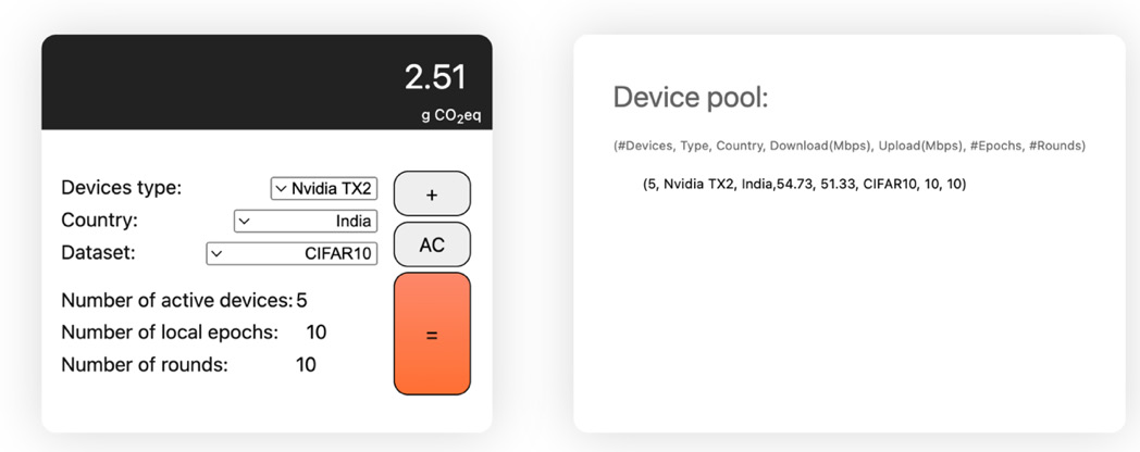
Figure 12.1 – Carbon emissions from an FL setup with 5 clients with 10 LEs and 10 rounds

Now, let us see how we compute the CO2e for centralized learning.

Centralized learning carbon emissions calculator

Just as with FL, we can do the same for centralized learning, as illustrated in Figure 12.1, using an ML CO2 impact calculator (https://mlco2.github.io/impact/ or https://github.com/mlco2/codecarbon) for different cloud platforms.

We also demonstrate in the following example how to measure carbon emissions using the CodeCarbon tool, which can easily be integrated with a natural workflow. It captures emission metrics from within the code and can help developers to track metrics at the function or module level:

1. As the first step, let us import all the necessary libraries:

   import tensorflow as tf
   from codecarbon import EmissionsTracker
   from tensorflow.keras.wrappers.scikit_learn import KerasClassifier
   from sklearn.model_selection import cross_val_score, StratifiedKFold,RandomizedSearchCV

   CopyExplain
2. In the next step, the following code demonstrates training a DL model using the MNIST dataset:

   def train_model():
       mnist = tf.keras.datasets.mnist
       (x_train, yv_train), (x_test, y_test) = mnist.load_data()
       x_train, x_test = x_train / 255.0, x_test / 255.0
       model = tf.keras.models.Sequential(
           [
               tf.keras.layers.Flatten(input_shape=(28, 28)), tf.keras.layers.Dense(128, activation="relu"),
               tf.keras.layers.Dropout(0.2),
               tf.keras.layers.Dense(10),
           ])
       loss_fn = tf.keras.losses.SparseCategoricalCrossentropy(from_logits=True)
       model.compile(optimizer="adam", loss=loss_fn, metrics=["accuracy"])
       model.fit(x_train, y_train, epochs=10)
       return model

   CopyExplain
3. Lastly, with the following code, we can track the emission numbers for training the DL code:

   with EmissionsTracker(project_name="mnist") as tracker:
       model = train_model()
   print(tracker.final_emissions)

   CopyExplain

Here is the output in kg CO2:

0.0001063754808656955

We can see that the DL model produces .0001063 kg of CO2 emissions.

We are now equipped with sustainable ML metrics for controlling our energy consumption. However, research has revealed that FL plays an important role in controlling CO2e emissions in different circumstances. Let us now see how we can incorporate sustainability during model training and deployment using FL.

With an exponential rise in ML training, over 300,000x from 2012 to 2018 – that is, with a 3-4-month doubling period (well exceeding Moore’s 2-year doubling period) – data scientists and algorithm researchers have increasingly investigated decentralized approaches of model training to try and curb the tremendous heat generated from DL models running on specialized hardware accelerators in data centers. This specialized hardware uses enormous amounts of energy (200 Terawatt-Hours (TWh)), higher than the national electricity consumption of some countries and contributing to 0.3% of global carbon emissions (as cited in the journal Nature in 2018). For example, Google’s AlphaGo Zero and training NLP models have released tons of CO2e, demonstrating the urgency of adopting a decentralized mechanism.

The exponential rise in the number of mobile and IoT devices means that FL and its collaborative method of training have been instrumental in lowering power consumption and carbon emissions. Furthermore, it has been found that the design of FL has a greener environmental impact due to fewer carbon emissions when compared with centralized learning.

Now, let us understand the emission metrics in the model training process.

CO2e emission metrics

To quantify the effect of training DL models in data centers or edge servers, the true environmental impact can only be understood when we account for the following metrics, as energy consumption is truly translated into CO2e emissions based on geographical location:

• The total amount of energy consumed by the hardware for both centralized learning and FL systems, along with the communication energy for FL systems
• The amount of energy consumed by the data centers due to cooling effects, particularly in the case of centralized learning

Now, let us isolate the factors that are responsible for energy consumption for centralized learning and FL-based training factors.

Comparing emission factors – centralized learning versus FL

The following factors summarize the principal differentiating points between energy consumption in centralized learning versus FL.

Hardware dependency

The energy consumption in the training process for centralized learning can be derived by sampling the GPU and CPU power consumption at training time. The NVIDIA System Management Interface can be queried to average the GPU power consumption of all samples during training. However, for FL, besides the aggregation server and clients equipped with a GPU, this part of energy consumption can be safely eliminated.

In an FL environment with a distributed training setup and multiple communication rounds from heterogeneous edge devices, the training time can far exceed that of centralized training. This is because centralized training converges much more quickly. For FL, the training time, and hence the energy consumption, is closely related to the number of clients selected in each iteration, the data distribution of clients (which is most often non-IID), and the heterogeneous client devices with varying computational power that take part in the training process, as clients exhibit varying computational power.

In addition to these factors, the actual energy consumed is also affected by the hardware devices (RAM or HDD) employed at each client device, the infrastructure, and the device distribution. When scaling FL setups, we need to carefully evaluate all the possible options before making the proper selection for the FL client’s hardware options. Hence, to differentiate the energy consumption metrics for centralized learning and FL, we need to benchmark the hardware for FL clients to validate the comparison metrics.

Data center cooling

The data center cooling process plays a significant role in overall energy utilization, with contributions reaching as high as 40% of the total energy consumed (Capozzoli and Primiceri, 2015: https://www.researchgate.net/publication/290010399_Cooling_Systems_in_Data_Centers_State_of_Art_and_Emerging_Technologies0). It is primarily dictated by the data center’s efficiency and estimated using the PUE ratio, which records an average of 1.67 for 2019 at a global level and is known for its variation across different cloud providers (recorded as 1.11 by Google, 1.2 by Amazon, and 1.125 by Microsoft in 2020). The FL training process does not have an associated cooling process. However, the central aggregation server can also be deployed with a cooling functionality.

Certain data center cooling techniques employ optimal control mechanisms through the use of hot/cold aisle arrangement (not separating hot and cold aisles to promote free air mixing), containment (by isolating hot and cold air), rack placement (to promote heat circulation from rack hotspots), cable organization (to allow uninterrupted airflow in the data centers), and the usage of blanking panels (to block hot air from entering the data center’s airflow). These are efficient cooling methods that sustain the temperatures in the data centers. Even deploying monitoring tools to manage the data center’s airflow, humidity levels, temperature, air pressure, and hotspots can result in greater efficiency due to better temperature and pressure control of the data center.

Energy utilization during data exchange

When training happens on a central server, there is certainly no data exchange involved. In contrast, in an FL ecosystem, the data and models are transferred, downloaded, or uploaded between the central aggregation server and the distributed clients. In addition to this, energy utilization also takes into consideration the energy utilized by routers and hardware on account of downloads and uploads.

Illustrating how FL works better than centralized learning

The result of experiments done by the Xinchi group (https://arxiv.org/pdf/2102.07627.pdf) explains, compares, and evaluates the impact of centralized learning versus FL:

• The number of target communication rounds needed to attain the target accuracy
• The energy associated with both centralized learning and FL
• The training times for both centralized learning and FL
• The different training optimizers used with FL

In the FL setup, each client was engaged in training a small dataset with low-power, GPU-enabled edge devices. The setup achieved the target accuracy within one or five LEs. In contrast, in a centralized training environment, one LE translates to a standard epoch, which was applied during the training process on the entire dataset.

Furthermore, it has been demonstrated that the energy utilization is even lower in an FL setup than in a centralized learning setup using an energy-efficient training optimizer such as FedAdam. FedAdam is well known for demonstrating faster initial convergence than Federated Averaging (FedAvg) and even performing better than FedAvg along with non-adaptive optimizers. This adaptive optimization technique does not result in additional client storage or communication costs but rather ensures compatibility with cross-device FL.

In FedAvg, clients engaged in training do so through several Stochastic Gradient Descent (SGD) steps to share local updates to the server. This method underperforms in heterogeneous settings (such as NLP domains with different users and different vocabularies) as it uses a simple average of the shared update to upgrade the initial model.

A gradient-based optimization technique such as FedAdam focuses on an adaptive server optimization procedure using per-coordinate methods to average the clients’ model updates. Here, the optimization at the server end aims to optimize the aggregated model from a global perspective using FedAvg and server momentum. On the other end, individual clients use a client optimizer over multiple epochs during local training. In this way, it minimizes the overall loss of local data during its limited participation process.

In FL, more often than centralized learning, a higher number of LEs results in the faster convergence of ML models in fewer FL rounds. Even though it does not ensure lower energy utilization, adaptive aggregation strategies such as FedAdam work better in terms of global model convergence speed.

In addition, non-IID datasets need more FL rounds than IID datasets, which converge more quickly than non-IID datasets.

The effectiveness of the FedADAM optimizer is evident in the Xinchi group study (the experiments illustrated are taken from the research results of A First Look into the Carbon Footprint of Federated Learning, https://arxiv.org/pdf/2102.07627.pdf), where we see that it performed better than FedAvg for both the CIFAR-10 and SpeechCmd datasets. Furthermore, using five LEs, the amount of CO2e emissions using FedAdam was lower than for centralized learning and FL using FedAvg. For ImageNet experiments, to achieve the required test accuracy in the non-IID data case, the emissions were higher in FedAdam than FedAvg. This happened because the dataset is naturally unbalanced, which leads to rounds of training being required to reach the target test accuracy. This contributes to longer training times, leading to a higher level of CO2e emissions. For example, the IID SpeechCmd dataset exhibits significantly lower emissions using the FedAdam optimizer.

Thus we see energy efficiency is dependent on a number of factors in both centralized learning and FL, a primary one being the optimizer used in FL. It is often possible, with non-IID datasets (for example, SpeechCmd) with the FedAdam optimizer, less complex model architectures, and fewer communication rounds, that FL yields lower CO2 emissions than centralized learning. Thus we can conclude that with lightweight neural networks employed, FL appears to be a better choice in terms of energy efficiency than centralized learning.

Let us understand how we can bring down CO2 emissions by making a trade-off and optimizing the following factors in FL.

The CO2 footprint of FL

Some of the leading factors in deciding the CO2 footprint of centralized learning and FL training are as follows, resulting in varying levels of CO2e emissions:

• Geolocation of hardware: For example, training in France has been found to produce the lowest CO2e emissions, as nuclear energy is the main source of energy in France, which consequently leads to the lowest energy-to-CO2e conversion rate.
• The type of DL model, specifically the model architecture: For example, FedAvg-based FL optimizations have been found to emit more CO2 for image-based tasks using ResNet-18 than modern GPUs and centralized training. The same FL-based optimizations have been found to emit less CO2 on the SpeechCmd dataset when training an LSTM model. If the local training tasks on FL are lightweight, with less communication and data exchange, studies demonstrate that it will lead to lower CO2 emissions.
• Hardware efficiency: Chips such as Tegra X2 are likely to be embedded into smartphones, tablets, and other IoT devices. FL will continue to reduce emissions when using this type of advanced chip.
• Cooling needs and availability in data centers: FL does not have a centralized cooling process in a data center; those cooling requirements are distributed across the devices included in the federation and vary based on each device’s needs. Distributed setups of centralized learning need a cooling facility. Advanced GPUs or TPUs (short for Tensor Processing Units) requiring high computational power demand more requirements for cooling and, consequently, high energy utilization.
• Communication rounds for FL: One LE in centralized learning yields more CO2 than five LEs, irrespective of the aggregation strategy or the device in place. This happens due to the fact that a lower number of local training epochs causes increased time for the model to converge. This ultimately leads to more data exchange and communication rounds between the local clients and the global server. With five LEs, individual devices train for longer, leading to fewer communication rounds and lower emissions.
• Data exchanges in FL: As we have seen before, the percentage of CO2e emission is also primarily driven by Wide-Area Networking (WAN) emissions due to exchanges between datasets and FL setups. For example, the energy utilization of communication may yield up to 0.4% (ImageNet with five LEs) and 95% (CIFAR-10 with one LE) of total emissions.

To bring parity and equivalency when comparing CO2e emissions, the communication rounds in FL are converted into centralized epochs. CO2e emissions are directly correlated to the number of centralized epochs. Some of the key factors in the increase in CO2 emissions put forward by the Xinchi group are as follows:

• The number of centralized epochs
• The thermal design power of hardware
• An increase in the model size, increasing the energy used for communication
• The size of the training dataset
• The use of a better DL-based optimizer, such as FedAdam, which can outperform centralized learning

We know how the devastating impacts of climate change over the last decade have required us to rethink and reconsider our emission metrics before deploying an architecture. Climate change and concern for a greener planet will drive research and innovation when designing new metrics. All these factors, when assembled, motivate us to choose better hardware that can provide visibility into the CO2 footprint and offer recommendations for possible remediations. It is now important for us to know how we can deploy popular design patterns for training FL models.

We should also look at other ways of generating energy from renewable sources, which can play an important role in convincing organizations to control their emissions and encourage investment in renewable energy.

Hence, let us walk through ways to compensate for CO2e emissions.

How to compensate for equivalent CO2e emissions

To compensate for CO2e emissions, we need to understand how the information regarding the energy grid or the conversion rate from energy into CO2e can be handled. As there is also a dearth of public sources of information, there are certain recommended practices to bear in mind:

• We must move with the assumption that all data centers and edge devices connected to a local grid are directly associated with their physical location. Electricity-specific CO2e emission factors are expressed in kg CO2e/kWh, with varying factors associated with each country, such as in France (0.0790), the US (0.5741), and China (0.9746).
• The emission technology (with suitable metrics to compute the energy lost when transmitting and distributing electricity) and the throughput or productivity of heat plants can impact the overall energy utilization.
• Evaluating the conversion factor for both FL and centralized learning with the aforementioned assumptions in mind can help us compute and target an energy utilization metric that has the least CO2 emissions. In FL, the energy used for communication varies based on the type of data partitions (more energy is required for IID datasets), the number of communication rounds, the hardware type, the location, and other factors that we have discussed.
• Our next goal as sustainability experts is to compensate for the resultant CO2 emissions by allocating renewable energy sources through buying Renewable Energy Credits (RECs) in the US or Tradable Green Certificates (TGCs) in the EU. Even initiatives to support environment-friendly projects, such as renewable energy initiatives or massive tree-planting activities, can be encouraged.

We now need to consider how we train FL models by considering different parameters that impact CO2 emissions.

Design patterns of FL-based model training

Till now, we have been concentrating on how FL is a great methodology from a sustainability standpoint. However, apart from sustainability, FL also offers a great benefit from a data privacy standpoint, in relation to Responsible AI. In FL, clients are able to share anonymized learning from their local data, instead of having to share potentially sensitive data with a centralized process. We will learn more about this in this section as we learn more about the different design patterns of FL.

FL has different design and deployment strategies that will impact its CO2 emission metrics. Some of the key metrics are as follows:

• The size of the non-IID datasets in each client
• The number of participating clients
• The wait time before clients engage in training that impacts the model convergence
• The training time for local clients and the time to aggregate the global model

Let us now see the different modes of FL-based training.

When we think about model training and data processing patterns using FL, we need to consider the type of data, along with the motivation of the clients to participate in local training. Hence, we can primarily divide them into three types:

• A multi-task model trainer to train non-IID datasets
• A heterogeneous data handler known for training heterogeneous datasets
• An incentive registry, which motivates clients through a reward system

In each of the illustrated figures corresponding to each of the design patterns, we used the sequence of FL, which is as follows:

1. A generic global model is trained by the central server.
2. Each client selected in the specific training round downloads the global model and kicks off the local training process.
3. The locally trained model from the client end is then updated on the global server.
4. The server aggregates the global models using the FedAvg algorithm to improve the shared version of the model.
5. The local devices are then updated with the newly retrained global model, which prepares them for local retraining and updates them for successive iterations.

The multi-task model trainer

This mode of training has the primary objective of improving learning efficiency and model performance metrics. Furthermore, it is most suitable for training separate related models on local devices. Specifically, we use this when the data distribution patterns of clients differ and the global model falls short of representing the data pattern exhibited by every client. For example, as the following figure illustrates, training separate models on computer vision, reinforcement learning, speech recognition, and NLP is essential for modeling and demonstrating the purpose of each model:

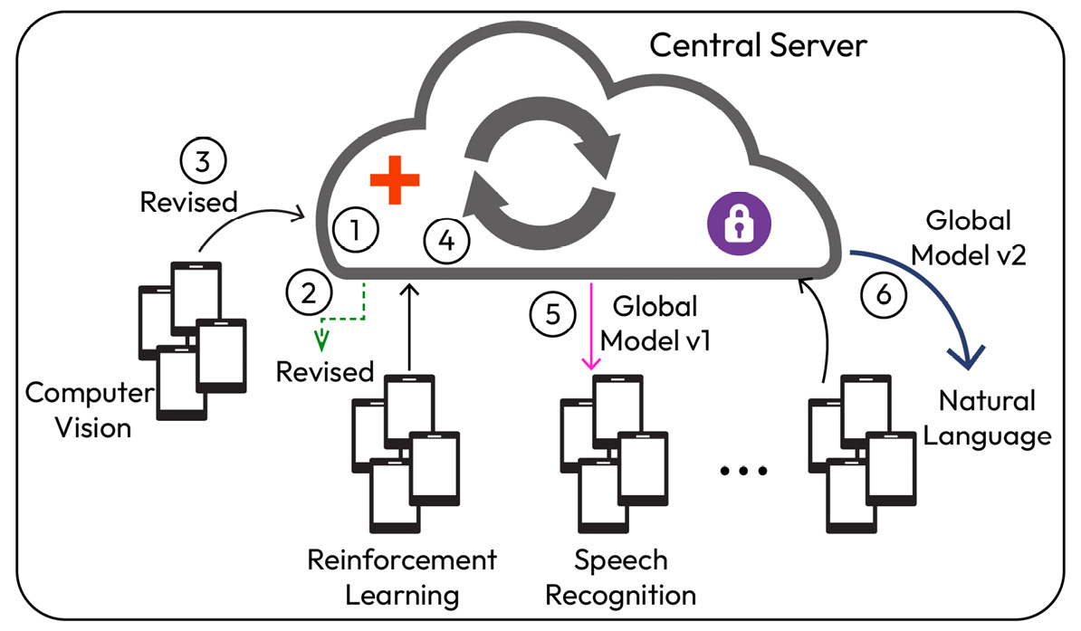
Figure 12.2 – FL model training design pattern – a multi-task model trainer

One real-world example would be to use ML to solve a next-word prediction task (performs related machine learning tasks involving NLP) by using device data such as text messages, web browser search strings, and emails.

To obtain higher accuracy, this design involves more training time, computation, and energy resources in every round, as expected with other conventional FL techniques. The major challenge of this method is the vulnerability of local clients to data privacy threats and the limitations of the training to convex loss functions.

A heterogeneous data handler

This mode of training preserves data privacy and finds better vanilla FL usage with non-IID and skewed data distributions by applying special processing techniques such as data augmentation and adversarial training with a generative adversarial network:

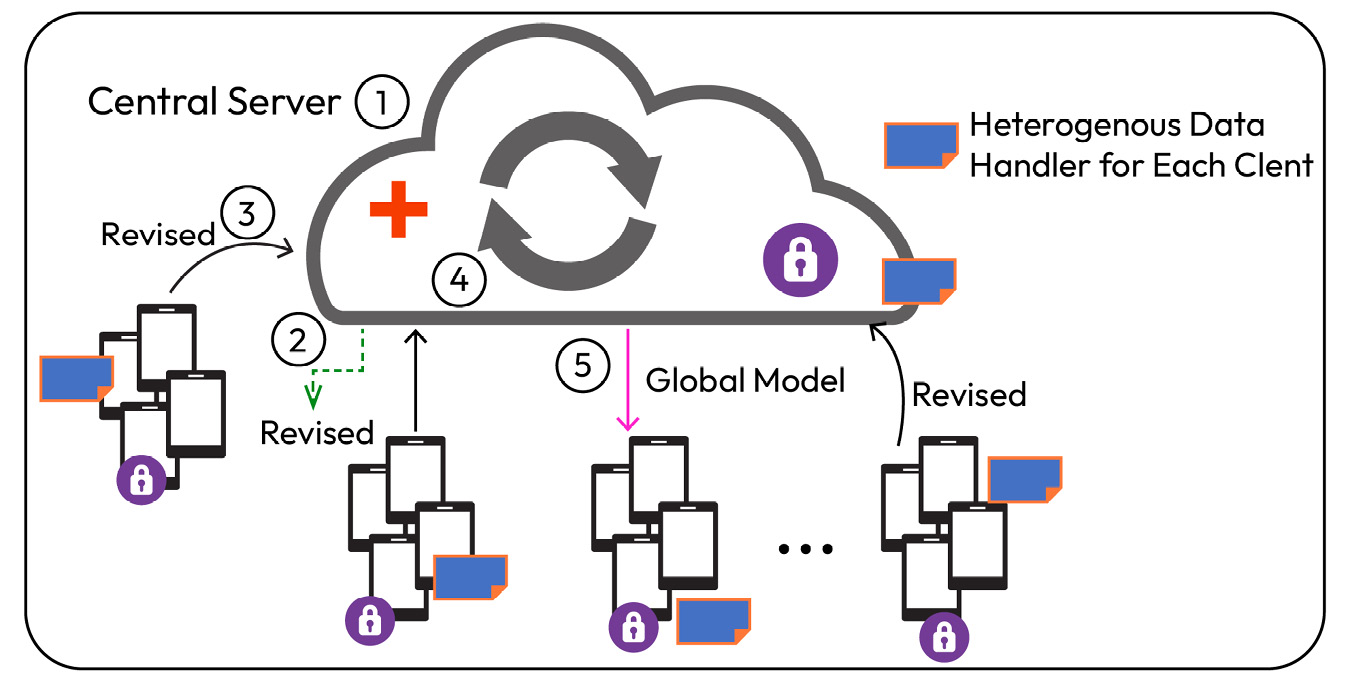
Figure 12.3 – FL model training design pattern – a heterogeneous data handler

As the personalized data of clients results in imbalanced and skewed data distributions, local models trained on devices tend to lower the global model accuracy upon aggregation. Hence, it becomes essential to promote data efficiency by plugging in a heterogeneous data handler that can correctly augment and distill the federated data and still preserve data privacy. The distillation process equips the client devices to gather information from other participating devices at intervals without any direct access to other clients’ data.

This mechanism tries to yield better model performance metrics at the cost of the training time and computational resources, which, ultimately, results in lower energy efficiency and a lower sustainability metric.

An incentive registry

The training model shown in the following figure rewards each participating client based on their contribution in terms of data volume, model performance, and computation resources, among other things. This is a measure to motivate clients and improve the performance of the global model. The following figure demonstrates a blockchain and a smart-contract-based incentive mechanism:

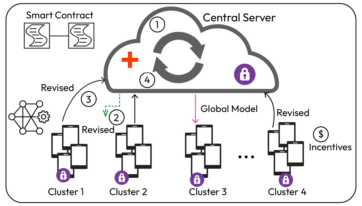
Figure 12.4 – FL model training design pattern – an incentive registry

Motivation energizes more clients to participate, as this training strategy is not driven by the complete participation of each and every client in every iteration. Moreover, the incentive scheme needs a mutual agreement between the clients and the learning coordinator to decide the evaluation criteria. Some of the common ways to formulate incentive schemes are reinforcement learning, blockchain/smart contracts, and the Stackelberg game model. One specific employment of blockchain-based FL incorporating incentives is FLChain, which supports collaborative training and a marketplace for model trading. This model also suffers from the challenge of long training times and computation resources.

In this section, we learned about important factors that control the FL training setup, including the parameters, the number of clients, time, and the epoch period of training. All these factors contribute to the energy used in training environments, which contributes to global warming. Beyond model training, let us also learn how different modes of model deployment also have an impact on energy emissions. In the following section, we will primarily discuss a strategy in an FL environment in which only selected clients are engaged in training. Although we will refer to individual clients taking part in the training process, our main goal is to understand the operational or deployment modes that enable clients to trigger the local training process.

Sustainability in model deployments

In the previous section, we learned how FL plays an important role in sustainability. Now, let us explore a sustainable ML framework for FL. We will see how to use rechargeable devices that are capable of accumulating energy from the ambient environment and effectively utilizing it during intermittent training periods.

This kind of framework can be extended to cross-device and cross-silo FL settings, including FL in wireless edge networks, IoT, and the Internet of Medical Devices (IoMD). Individual local device training can drive model convergence, as well as make it adaptable to the following settings:

• Enabling the random selection of a small number of clients to minimize the communication overhead during every iteration.
• Enabling the selection of clients to maximize the learning rate to speed up the convergence rate.
• Enabling a client selection process based on the energy arrival process at each client. This is to address intermittent and non-homogeneous energy arrival patterns to effectively manage clients dropping out.

This deployment framework can rightly fit scenarios in which heterogeneous devices are available and each training round works independently. This makes the framework much more flexible, as each device participating in the training process in one round is not held accountable or dependent on future consecutive rounds. The training process (driven by random energy availability) is coordinated by the central server, which aggregates the local models of the clients to send them the updated global model. The individual clients are engaged in the local training with their own datasets, as well as updating the global model received using multiple SGD iterations over their local dataset. The framework not only benefits from energy-efficient sustainable FL training but also minimizes the total energy cost of training in scenarios where devices generate energy through an intermittent and non-homogeneous renewal process.

The framework allows clients of different types to have varying levels of energy generation to participate in training, with two different configurations:

• A biased model prediction strategy, where the global model is biased toward clients that have more frequent energy availability. This kind of model sees a performance loss in the accuracy of the predicted outcomes but yields a better convergence rate.
• An unbiased model prediction strategy, where there is a wait associated with letting all the clients generate enough energy before each iteration of participating in the training process. This kind of model suffers from the longest wait time based on the slowest client. However, this kind of training has better performance metrics, despite having a slow convergence rate.

The proposed framework is equipped with four different entities, as described here, to facilitate an energy-aware client scheduling and training strategy:

• The energy profile of clients: Accounting for the energy availability of all clients is the most important factor, as it governs the client participation based on the energy received from the ambient environment, such as solar, kinetic, ambient light, or RF energy. Profiling is a mechanism for studying energy patterns to infer the availability of sufficient energy to train the local model and send updates to the central server. Any participating client starting the training process at a global round starting at the initial time instant t ensures the client participates for the whole duration of that global round, {t, . . ., t+T −1}, where the client is engaged in training the local model. In addition, clients taking part in the training process for any global round remain constant during the entire duration of training for that specified global round.
• Client scheduling: The framework comes with the flexibility of allowing clients to decide whether they want to participate in the training process at that specific iteration based on their energy profile. The stochastic participation process incorporates clients after locally estimating the energy arrival process to maximize the convergence rate or reduce the communication overhead of training. The scheduling process does not necessitate coordination among clients, making it easier to scale in large networks.
• Local training at the client: This phase allows participating clients to train their local datasets using SGD and then update them on the central server.
• Model updates by the server: This phase allows the server to aggregate the local models to consolidate the global model to be sent to individual devices.

Having studied the principal influencing factors behind energy-intelligent client scheduling, here, we will discuss how the scheduling process works based on the energy availability of clients.

Figure 12.5 illustrates the two different prediction strategies, where clients either take part as soon as energy arrives or wait until all clients have accumulated the energy required to start training. The left-hand part of the figure is optimistic about model convergence and starts client scheduling immediately when the energy is available (as represented by different colors of t1, t2, t3, and t4). On the other hand, the right-hand subfigure is conservative and waits until energy is available for all the clients to schedule them together, as represented by them all being the same color, orange, where t1, t2, t3, and t4 are different time instances:

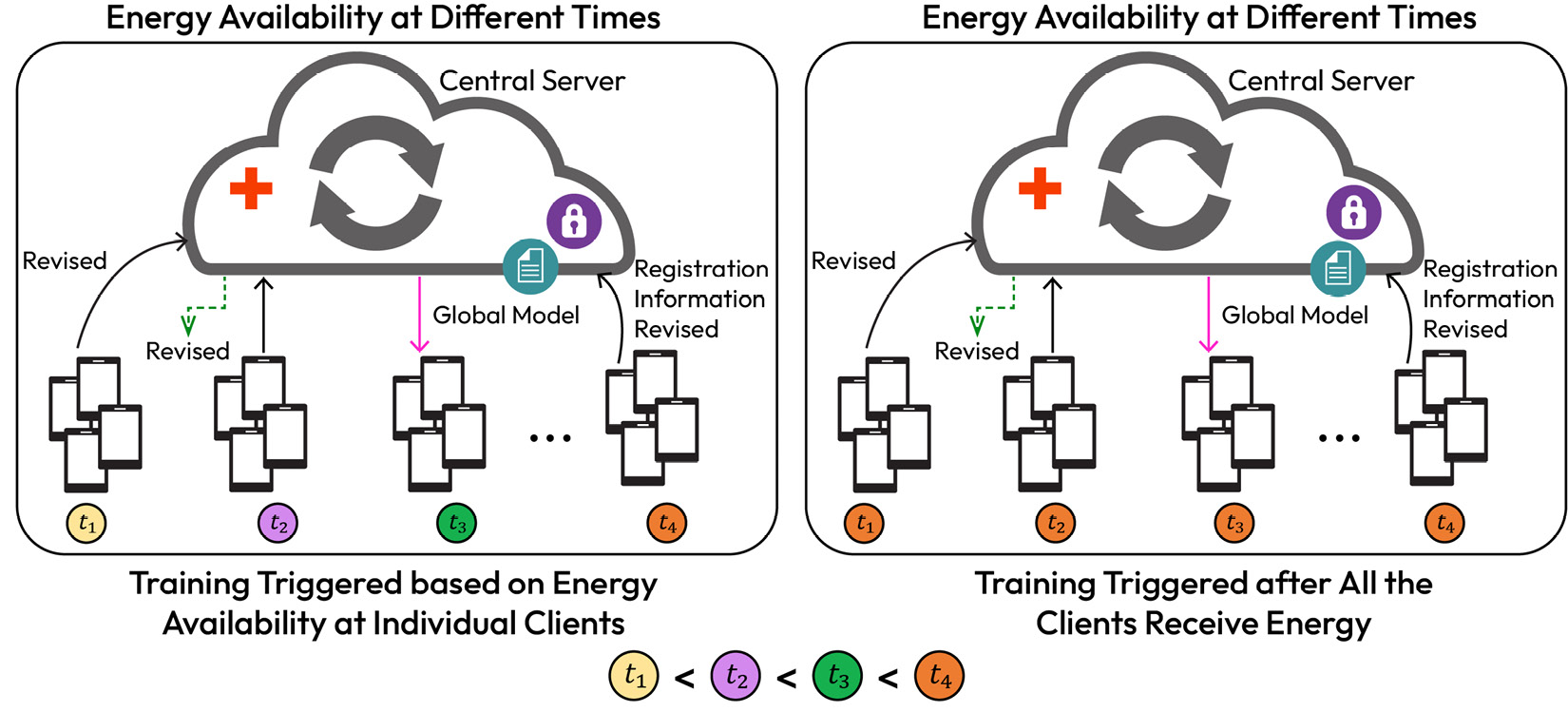
Figure 12.5 – Client scheduling based on energy arrival patterns

In this section, we have learned how sustainable FL can be deployed in large-scale networks using stochastic energy arrival processes. Furthermore, adapting model quantization and compression techniques with a completely random energy availability among clients promises a better characterization of the relationship between the energy renewal processes and the training performance.

We have understood scheduling the client’s training process based on energy. Now, let us see how these training patterns can be scheduled according to the architecture and how to scale FL models.

Design patterns of FL-based model deployments

Let us deep-dive into how FL models can be managed and aggregated once they are live in production. Here, we will discuss two types of architectural designs that come into play, mainly from the perspective of data communication, model management, and governance, and how these models are aggregated and distributed to local clients:

• FL-based model management patterns: We need the model management patterns to establish the rules and processes related to the local client’s data or model size. The size plays a critical role in the data or model exchange and, hence, the amount of energy consumed. In addition, the frequency of replacing the model and updating the global model serves as a deciding factor in the CO2e and the sustainability of FL.
• FL-based model aggregation patterns: We need model aggregation patterns in FL to consolidate learning from individual clients to create an updated global model. The mode of the m­odel aggregation process from the deployed clients – be it asynchronous, hierarchical, or decentralized – impacts the timing and the latency. All these factors contribute to varying levels of CO2e.

Let us discuss these designs in the following sections.

FL-based model management patterns

Model management patterns are responsible for model transmission, deployment, and governance. Based on how messages are transferred or models are stored locally by clients, we can divide them into four broad categories, as described here:

• A message compressor, which reduces the transmitted message size
• A model co-versioning registry, involved in model version management by receiving model updates from clients, helping to facilitate model aggregation
• A model replacement unit, which monitors the global model’s performance and initiates new training when the model starts to show a reduced performance
• A deployment selector, which pushes the improved global model to the clients

Let us discuss each of these four categories in detail.

A message compressor

This design pattern, as demonstrated in Figure 12.6, compresses the message to reduce its data size during the model exchange process during every round:

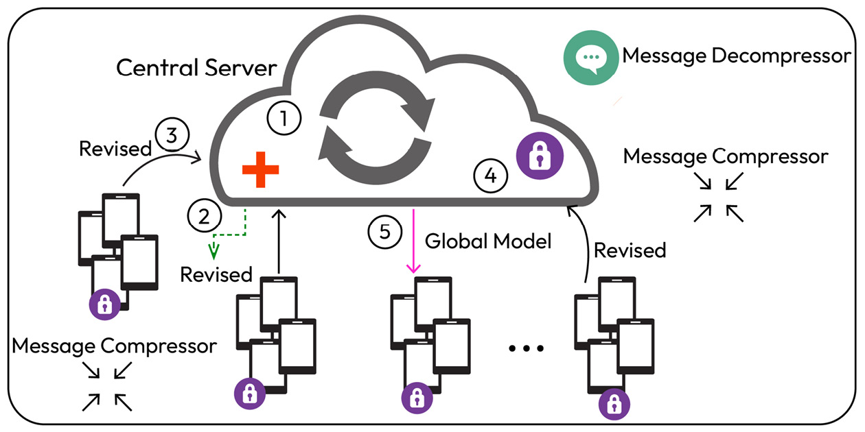
Figure 12.6 – FL model deployment design pattern – message compressor

This process helps to increase the efficiency of communication by effectively compressing model parameters or gradients in limited-bandwidth scenarios. However, the pattern incurs additional computation costs when the server must aggregate sizeable model parameters. Moreover, it also adds an overhead for message compression and decompression and may involve the loss of essential information.

A model co-versioning registry

The model co-versioning registry, as shown in Figure 12.7, aids the local model governance process by tracking each client’s model version and aligning it with the global model of that corresponding iteration:

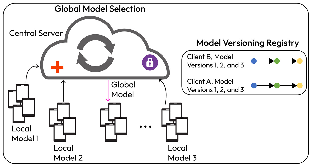
Figure 12.7 – FL model deployment design pattern – model co-versioning registry

This facilitates synchronous and asynchronous model updates, client dropouts, model selection, and stopping complex model training early. Furthermore, this pattern has the unique advantage of tracking the model quality (including global models, client device updates, and the version of the application or the device OS/firmware), and adversarial activities by clients (where a client acts as an adversary) to strengthen the accountability of the system. The registry is used to collect local model updates and map them to the global model so that the model version number and client IDs stay immutable. This pattern can also be implemented using a blockchain to provide model provenance and co-versioning. The added storage volume required by this architecture to store all versions of the global and local models comes with the increased benefit of offering system security to detect dishonest clients that may cause a system failure. One prime example of this pattern is the MLflow Model Registry built on Databricks, which has an efficient centralized model store for tracking the chronological model lineage, versioning, and stage transitions.

A model replacement trigger

This FL design pattern initiates the replacement of the model by setting a trigger on a new model task whenever the model’s performance degrades below an acceptable threshold. To address issues such as a drop in the model’s accuracy, this pattern provides mechanisms to investigate the reason for this reduced accuracy before establishing the new model training process. The retraining process is set only when the degradation in model performance is noticed for a few consecutive rounds to strongly infer that the performance reduction is global. Retraining the model adds a cost both in terms of communication and computation but is effective in handling clients in an FL environment with heterogenous non-IID datasets where clients have personalized datasets and exhibit faster decays in the global model’s performance over successive iterations. Microsoft Azure Machine Learning designer and Amazon SageMaker are well-known platforms for triggering model retraining based on the degradation of model performance.

A deployment selector

This deployment strategy, as demonstrated in Figure 12.8, enables the convergence of the global model and pushes the global model to selected clients based on the application on which they run. Hence, different groups of clients receive different versions of converged models, and this aims to improve the performance metrics of the models. The model selection addresses the non-IID data distribution among clients so that different customized converged models serve different groups of clients better. However, this procedure comes with added overhead on the server, as the central server needs to properly identify the clients to provide them with different versions of the global model and, at the same time, train and store different models for diverse clients. Despite the increased training cost, we get better-generalized models based on the ML task of the clients. This strategy needs to have extra privacy measures built in to prevent privacy leakage when the server tries to group clients. This type of FL training is available on Amazon SageMaker and Google Cloud, which trains and manages multiple model versions and deploys them at different endpoints:

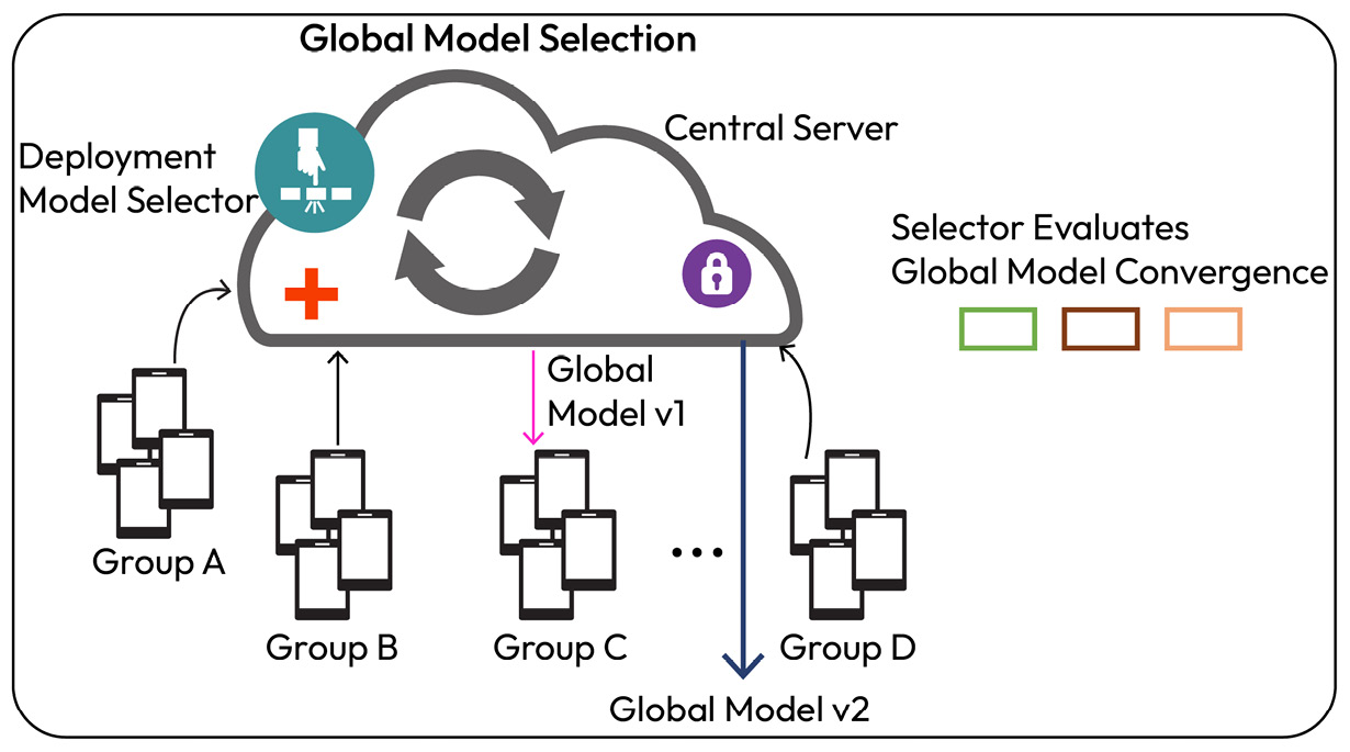
Figure 12.8 – FL model deployment design pattern – model deployment selector

FL-based model aggregation patterns

This design pattern employs different tactics for model aggregation to reduce aggregation latency and increase the system’s efficiency, reliability, and accountability. The primary objective is to improve the model performance metrics by effectively utilizing optimal resources. They can be broadly divided into the following four types of patterns:

• An asynchronous secure aggregator
• A decentralized aggregator
• A security aggregator
• A hierarchical aggregator

We have illustrated the four patterns in the following subsections; the last two patterns can be combined into a hybrid hierarchical secure aggregator.

An asynchronous aggregator

This asynchronous global model aggregation strategy, as shown in the following figure, enables us to speed up the model aggregation with the arrival of a new model update without waiting for the models that are trained locally the clients.

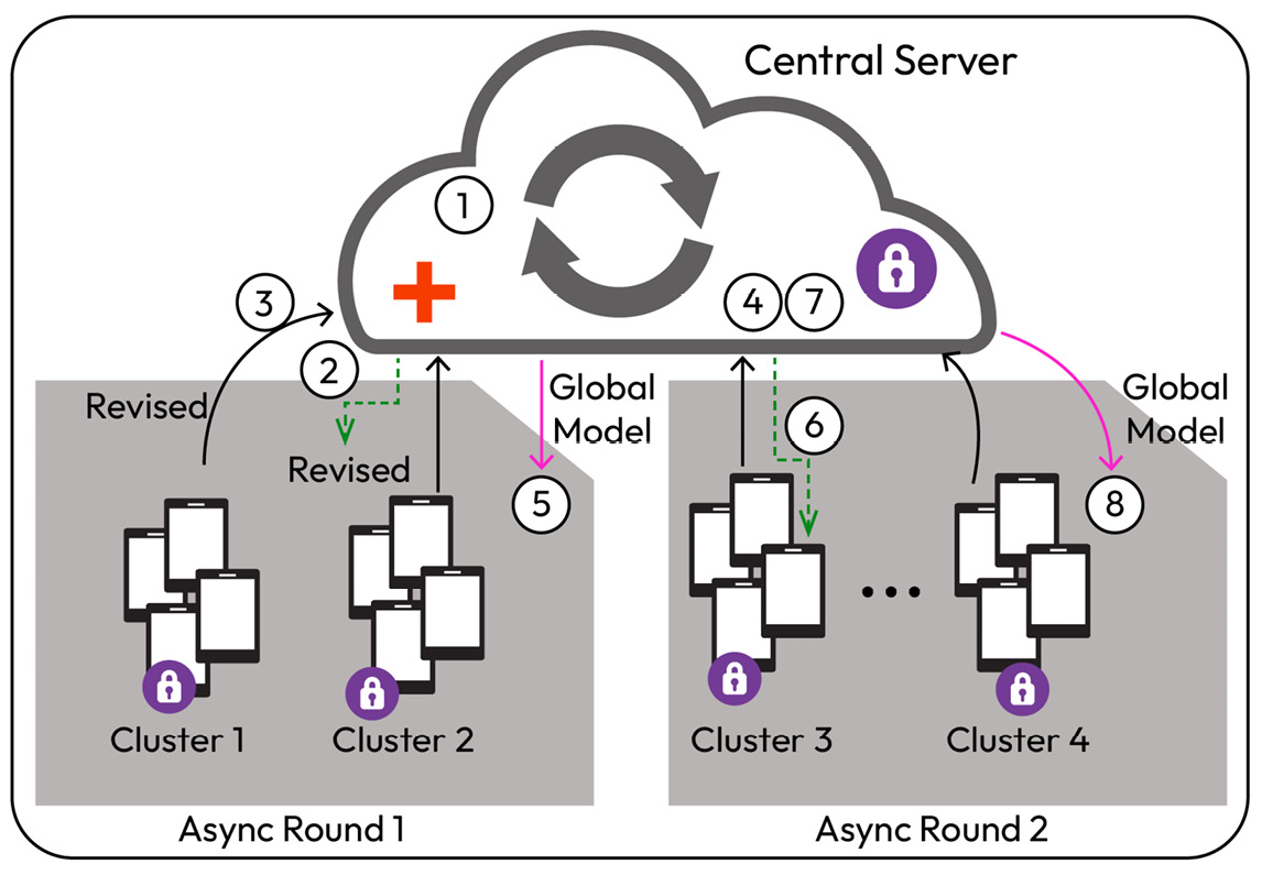
Figure 12.9 – FL model deployment design pattern – asynchronous aggregator

This mechanism differs from conventional FL by allowing clients to skip the first aggregation round, where clients engage in updating models asynchronously during the next (second or successive) aggregation phase. Hence, it accommodates the variability of clients in terms of their computational resources, bandwidth availability, and communication capacities. The clients enjoy a definite advantage when participating in global model aggregation where the model convergence process by the server is not impacted by delays.

The challenge of employing this strategy results in a bias in the global model, which may impact the model’s quality if important information is eliminated. In addition, the maximum aggregation latency at the server is dictated by when the slowest client sends the updates, leading to slow model convergence.

However, some of the key benefits include centralized aggregation happening at each round instead of waiting for the slowest client. We also see reduced bandwidth usage during each round, as few clients send their updates asynchronously.

Examples of design patterns include Asynchronous Online Federated Learning and Asynchronous Federated Optimization.

A decentralized aggregator

This aggregation strategy, as demonstrated in the following figure, follows a decentralized FL approach by removing the dependency on a central server that turns out to be the single point of failure. Here, the central server may experience additional loads, as it receives and aggregates updates from all clients. The figure illustrates how a blockchain and a smart contract can be used to receive model updates when updates are shared with neighboring devices. In conventional FL training, the system may suffer from privacy limitations when not all participating clients trust the central server.

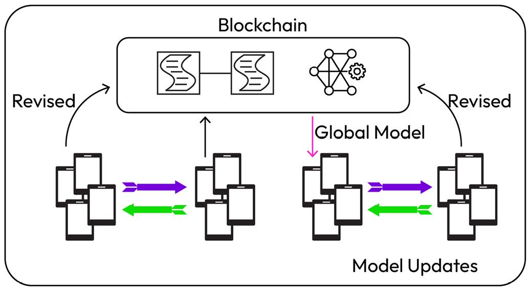
Figure 12.10 – FL model deployment design pattern – decentralized aggregator

This decentralized approach is recommended where model updates are allowed between peer client devices. However, this architecture also requires a proper definition of a decentralized model management system, where peer systems can collect, store, examine, and aggregate the local models. Moreover, we also need to define system ownership, through which a random client is selected to perform the aggregation from the local nearby clients and send the aggregated model to the client network. The blockchain serves as one of the best options for decentralized FL, where it can store immutable models and the learning coordinator can maintain the blockchain. A blockchain mechanism is reliable, accountable, and trustworthy, thereby increasing resiliency to adversarial attacks, trust, and transparency.

One of the major drawbacks of this system is the latency involved due to the blockchain consensus protocols during the model aggregation process. In addition, client devices may also experience power drainage due to their parallel participation in training and model aggregation. Even this kind of decentralized architecture runs the risk of clients exposing sensitive information about their peers to others. One practical example of this mode of peer-to-peer learning is BrainTorrent, in which clients engage in direct learning and communication with each other.

A security aggregator

This aggregation strategy supports built-in security protocols to protect the model better than vanilla FL without any support for data encryption. This is in contrast to conventional FL, which does not take data encryption and the secure exchange of parameters into consideration and leaves room for unauthorized data access. To prevent malicious clients from joining the training process and curb poisoning attacks on the data/model, we need to ensure that the proper security protocols are in place as and when models send updates to the central server. The best way to ensure that model parameters and gradients are not accessible to third parties is to employ secure, multi-party computation for model exchanges and aggregations to guarantee that each participating client is aware of its model input and output. We can also employ homomorphic encryption to allow the client to encrypt and the server to decrypt the model. Application-level security mechanisms such as pairwise masking and differential privacy help reduce data leakages to external adversaries.

Some of the drawbacks of this mode of architecture include the reduction in system efficiency and lower model accuracy at the cost of the addition of extra security protocols and encryption methods. Hence, we need to choose the right privacy thresholds to balance the trade-off between the model’s performance and privacy. The Secure Aggregation protocol (developed by Google) serves as one of the prime examples of a secured aggregation protocol in FL.

A hierarchical aggregator

This aggregation technique adds an extra hierarchical aggregator layer (such as an edge server) to reduce the impact of non-IID on the global model and increase the system’s efficiency. The following figure illustrates how we might employ edge network 1 and edge network 2 to carry out partial aggregation from nearby client devices before triggering the global aggregation process. This design pattern, with intermediate servers at the edge networks, has been introduced to handle slow communication between clients and distant servers to improve the system’s efficiency. Involving a hierarchical aggregator in the process helps scale FL systems and facilitates a better global model aggregation, as the server can assemble local models from clients that have similar data heterogeneity.

The main drawback of this kind of architecture is the system reliability when devices are disconnected from the edge servers, which impacts the model training and performance. In addition, we need to be extra cautious about the security protocols, as edge servers can have security breaches and are more often subjected to network security threats.

One real-world example of an FL model that directly uses this architecture is Hierarchical FedAvg, where multiple edge servers are employed for partial model aggregation depending on updates that are incrementally received from the clients:

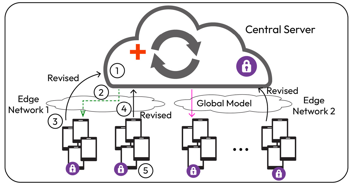
Figure 12.11 – FL model deployment design pattern – hierarchical aggregator

In this chapter, we have learned about the rising importance of sustainability when developing AI solutions, as well as the desired cloud metrics and architectural and operational know-how that can help us to reduce CO2 emissions. We saw a detailed overview of how FL models can be trained based on energy availability at the clients’ end to reduce the detrimental impact of higher CO2 emissions. We are now aware of efficient FL-based design patterns, whether training, model management, or model aggregation patterns.

In the context of training and deployment strategies for FL, we also got the chance to explore the benefits of different DL-based training optimizers and their impact on the sustainability of solutions. Furthermore, we walked through the sustainability factors in centralized learning versus FL, which can help us to estimate the CO2 footprint of the GPU compute using the specification of the type of hardware, its efficiency, the active runtime period, the model architecture, cooling needs, the cloud provider, and the region. We explored how to calculate the total energy consumed, the different emission metrics we can use, and the best practices we can follow to maximize our data centers’ efficiency.

In the next chapter, we will go deeper into exploring how to ensure sustainability while creating feature stores.

• Towards the Systematic Reporting of the Energy and Carbon Footprints of Machine Learning: https://jmlr.org/papers/volume21/20-312/20-312.pdf
• How Can I Calculate CO2eq emissions for my Azure VM?: https://devblogs.microsoft.com/sustainable-software/how-can-i-calculate-CO2eq-emissions-for-my-azure-vm/
• A Framework for Sustainable Federated Learning, B. Güler and A. Yener: https://dl.ifip.org/db/conf/wiopt/wiopt2021/WiOpt_2021_paper_100-invited.pdf, 2021 19th International Symposium on Modeling and Optimization in Mobile, Ad hoc, and Wireless Networks (WiOpt)
• Sustainable federated learning: https://arxiv.org/pdf/2102.11274.pdf
• Cloud sustainability: https://cloud.google.com/sustainability
• How carbon-free is your cloud? New data lets you know: https://cloud.google.com/blog/topics/sustainability/sharing-carbon-free-energy-percentage-for-google-cloud-regions
• CO2 in Federated Learning: https://mlsys.cst.cam.ac.uk/carbon_fl/
• Can Federated Learning Save The Planet? https://arxiv.org/pdf/2010.06537.pdf
• Architectural Patterns for the Design of Federated Learning Systems: https://www.researchgate.net/publication/348316341_Architectural_Patterns_for_the_Design_of_Federated_Learning_Systems