Hyperparameter Tuning, MLOps, and AutoML

Developing a Machine Learning (ML) model is an iterative process; the presence of so many models, each with a large number of hyperparameters, complicates things for beginners. This chapter continues from the previous chapter and explains the need for continuous training in ML pipelines. It will provide a glimpse of the AutoML options currently available for your ML workflow, expand on the situations in which no-code/low-code solutions are useful, and explore the solutions provided by major cloud providers in terms of their ease of use, features, and model explainability. This chapter will also explore orchestration tools such as Kubeflow and Vertex AI, which you can use to manage the continuous training and deployment of your ML models.

After completing this chapter, you will be familiar with the concept of hyperparameter tuning and popular off-the-shelf AutoML and ML orchestration tools.

In this chapter, these topics will be covered in the following sections:

Introducing AutoML
Introducing H2O AutoML
Working with Azure AutoML
Understanding AWS SageMaker Autopilot
The need for MLOps
TFX – a scalable end-to-end platform for AI/ML workflows
Understanding Kubeflow
Katib for hyperparameter tuning
Vertex AI

Technical requirements

This chapter requires you to have Python 3.8 installed, as well as certain Python packages, listed here:

TensorFlow (>=2.7.0)
NumPy
Matplotlib

You need to install H2O as follows:

pip install -f http://h2o-release.s3.amazonaws.com/h2o/latest_stable_Py.html h2o

Alternatively, you can install it this way:

conda install -c h2oai h2o

Install the Azure ML client library:
```
pip install azure-ai-ml
```

Introduction to AutoML

Anyone who has worked in the domain of ML can tell you that building ML models is a complex and iterative process. You start with a dataset and a set of features, and then train a model on that data. As you get more data, you add more features, and you retrain your model. This process continues until you have a model that generalizes well to new data. The task is complicated by the fact that there is a multitude of hyperparameters and that they have a kind of non-linear relationship to model performance. Choosing the right model and selecting the optimum hyperparameters is still considered alchemy by many.

Note

You can refer to Has artificial intelligence become alchemy? Matthew Hutson, Science, Vol 360, Issue 6388 for more information.

Whether AI is alchemy or not is a hot debate. While many who start experimenting with AI feel that it is alchemy, there are experts, including us authors, who believe it is not so. AI, like any other experimental science, is based on technological foundations. Initially, the focus of AI was on the development of AI models and architectures, but now the focus is slowly shifting toward responsible and explainable AI. As more and more work happens in this area, we will be able to understand AI just like any other technology.

Finding the right model, the perfect features, and the best set of hyperparameters can be a time-consuming and frustrating task. Automated ML (AutoML) helps you select a model and hyperparameters.

It allows start-ups and low-budget organizations to benefit from the power of AI without investing in expensive and difficult-to-find AI talent. Therefore, to reduce the barriers to ML and help experts from other domains to use ML in their tasks, the automatic generation of ML models has been investigated by most major players working in the ML domain.

Broadly, we can divide building AI models into the following three iterative processes. This is illustrated in Figure 6.1:

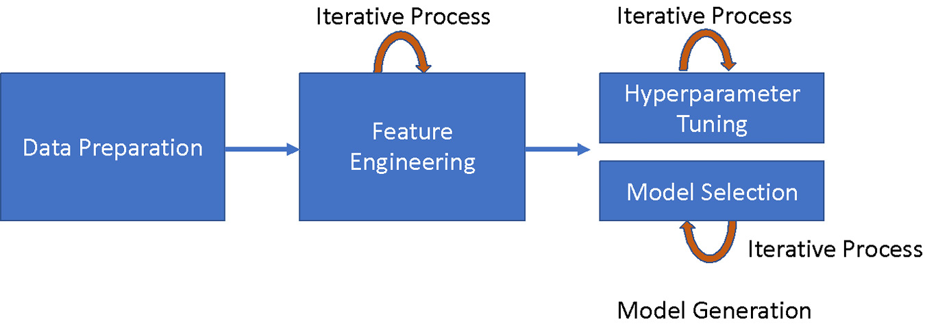
Figure 6.1 – The iterative processes in the ML pipeline

Let’s discuss each one:

Feature engineering: Feature engineering is an essential part of the ML process. Simply put, it is the process of creating and selecting (new) features from existing data that can help with model training. This can be done in several ways, but the most common methods involve either transformation or aggregation. Transformation involves transforming existing data into a new form, such as converting text into numerical values. Aggregation involves combining multiple data points into a single value, such as taking the average of a group of numbers. Feature engineering can be time-consuming, but it is often essential for building accurate models. With careful planning and execution, it is possible to create powerful features that can make all the difference to your ML results.
Hyperparameter tuning: This is the process of optimizing an ML algorithm by fine-tuning the hyperparameters to obtain better performance. The hyperparameters are a set of variables that control the model training process. They differ from the parameters of the ML models (for example, weights and biases in neural networks), which are learned during the training process. Hyperparameter tuning is crucial in any ML project, as it can significantly impact a model’s performance. However, it can be a time-consuming and expensive process, especially for large and complex datasets. There are various methods for hyperparameter tuning, including manual tuning, grid search, and random search. Each method has its advantages and disadvantages, and it is essential to select the right method for the specific problem at hand.
Model selection: Model selection is the process of choosing the ML algorithm that is best suited to a specific task. There are many factors to consider when selecting a deep learning model, such as the type of data, the desired output, and the computational resources available. The model selection process can be daunting. In the last few years, deep learning models have developed near-human performance in specific tasks. Many of these models were carefully crafted by AI experts, and the process of finding the model and its optimum architecture was not straightforward. Instead, it involved much human intuition and many trials and failures.

Domain experts unfamiliar with deep learning technologies can easily use AutoML to create ML solutions. AutoML is designed to simplify the process of creating ML models and reduce the expenses of building ML solutions by hand, which it does by automating the complete ML pipeline, including data preparation, feature engineering, and automatic model generation. Ultimately, the goal of AutoML is to make deep learning more accessible to everyone so that we can all benefit from its power.

Automating the creation and tuning of ML end-to-end pipelines offers simpler solutions. It helps reduce the time to produce them and ultimately might produce architectures that could outperform models crafted by hand. It is an active and open research area, with the first research paper on AutoML published at the end of 2016.

Most commercially available AutoML platforms take structured data and assume that data preparation and feature engineering have already been done, but they still offer model generation. Model generation can be divided into two parts – the search space and optimization methods. The search space identifies the different model structures (such as support vector machines, k-nearest neighbors, and deep neural networks) that can be designed, and optimization methods refine the chosen model by adjusting its parameters to improve its performance. Automated Neural Architecture Search (NAS) is gaining much attention nowadays. In their survey paper, Elsken et al. divide NAS into the following three major components:

Search space: This consists of a set of operations and how these can be connected to make a valid network architecture.
Search algorithms: This involves algorithms that are used to find a model architecture with high performance in the search space.
Model evaluation: This involves predicting the performance of the proposed models.

Figure 6.2 provides an overview of the NAS pipeline, listing various methods, algorithms, and strategies employed in the process:

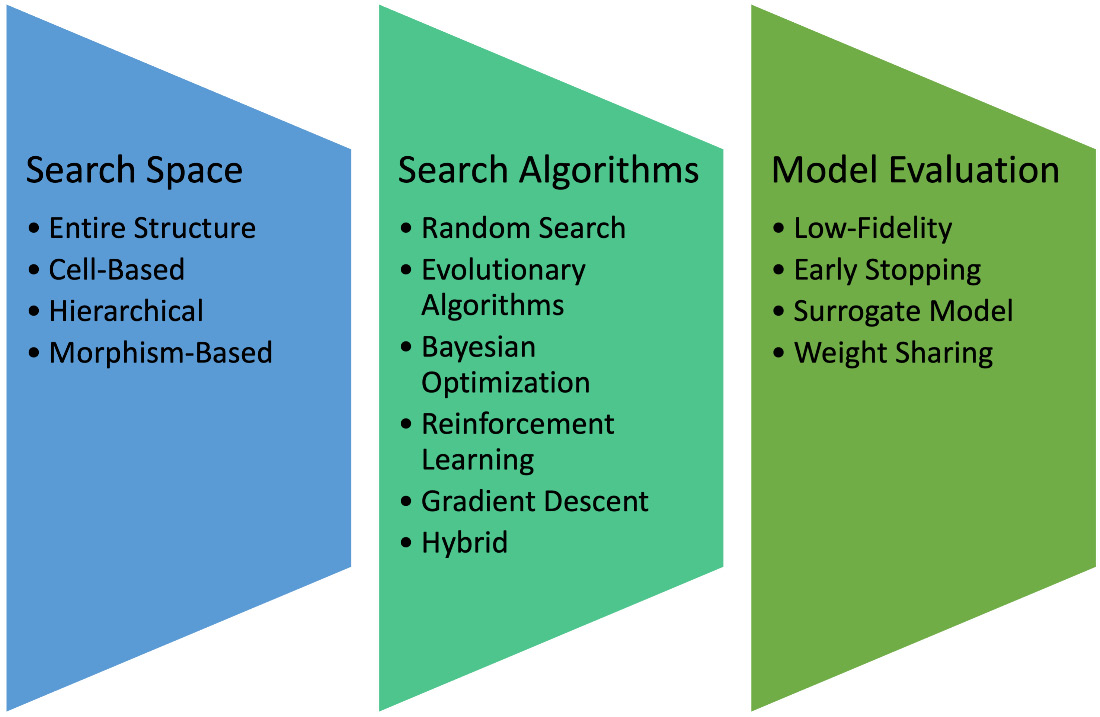
Figure 6.2 – An overview of the NAS pipeline (adapted from Figure 5 of AutoML: A survey of the state of the art, Xin He et al., Knowledge-Based Systems 212 (2021): 106622)

Let’s now explore some of the platforms offering AutoML services.

Introducing H2O AutoML

H2O is a fast, scalable ML and deep learning framework developed by H2O.ai, released under the open source Apache license. According to the company website, at the time of writing, more than 20,000 organizations currently use H2O for their ML/deep learning needs. The company offers many products, such as H2O AI Cloud, H2O Driverless AI, H2O Wave, and H2O Sparkling Water. In this section, we will explore its open source product H2O AutoML.

H2O AutoML is an effort to create a user-friendly ML interface that beginners and non-experts can utilize. It automates the process of training and tuning a wide range of candidate models. The interface is designed in a way that users only need to specify their dataset, the input and output features, and any limitations on the number of total models trained or time constraints. The rest of the work is done by AutoML; it recognizes the best-performing models within the specified time period and provides a leaderboard. It is often observed that the stacked ensemble model, an ensemble of all the previously trained models, typically holds the top position on the leaderboard. Advanced users have countless options to choose from; details of these options and their various features are available at http://docs.h2o.ai/h2o/latest-stable/h2o-docs/automl.html.

You can learn more about H2O on their website: http://h2o.ai.

Let’s try H2O AutoML on synthetically created data. Before you start, make sure you have H2O installed:

Using scikit-learn’s make_circles method, we first create a synthetic dataset and save it as a CSV file:

from sklearn.datasets import make_circles
import pandas as pd
X, y = make_circles(n_samples=1000, noise=0.2, factor=0.5, random_state=9)
df = pd.DataFrame(X, columns=['x1','x2'])
df['y'] = y
df.head()
df.to_csv('circle.csv', index=False, header=True)

Next, we initiate the H2O server – before we can use H2O, this is an essential step. This can be done using the init() function:
```
import h2o
h2o.init()
```

Once the H2O server has been initialized, it will show details about the H2O cluster, as shown in Figure 6.3:

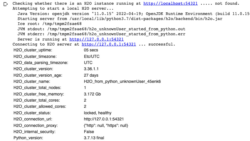
Figure 6.3 – Output of the H2O init command

Next, we read the file containing the synthetic data we created earlier. Since we want to regard the problem as a classification one, whether the points lie in a circle or not, we redefine our label of y as asfactor() – this will tell the H2O AutoML module to treat the y variable as categorical and, thus, the problem as a classification one. The dataset is split into training, validation, and test datasets in a ratio of 60:20:20:
```
class_df = h2o.import_file("circle.csv",
                    destination_frame="circle_df")
class_df['y'] = class_df['y'].asfactor()
train_df,valid_df,test_df = class_df.split_frame(ratios=[0.6, 0.2],
                   seed=133)
```
Now, we invoke the AutoML module from H2O and train it on our training dataset. AutoML will search a maximum of 10 models – you can change the max_models parameter to increase or decrease the number of models to test:
```
from h2o.automl import H2OAutoML as AML
automl = AML(max_models = 13, max_runtime_secs=75, seed=27)
automl.train(training_frame= train_df, 
        validation_frame=valid_df, 
        y = 'y', x=['x1','x2'])
```

For each of the models, H2O provides a performance summary. For example, in Figure 6.4, you can refer to the evaluation summary for BinomialGLM:

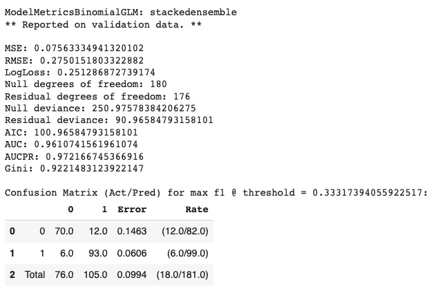
Figure 6.4 – The performance summary of one of the models by H2O AutoML

You can check the performance of all the models evaluated by H2O AutoML on the leaderboard:
```
lb = automl.leaderboard
lb.head()
```

Figure 6.5 shows a snippet of the leaderboard:

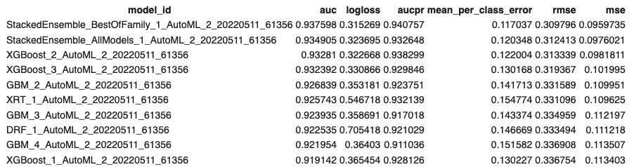
Figure 6.5 – Leaderboard summary – H2O AutoML

Besides AutoML, H2O also provides methods for explaining a model. Please refer to Chapter 9 and the Jupyter notebook on H2O in the book’s GitHub repository to learn more about the model explainability features provided by H2O.

Next, we will explore the Microsoft AutoML tool, Azure AutoML.

Working with Azure AutoML

Azure provides AutoML solutions for tabular, text, and image data. Azure uses Bayesian optimization to find the optimal model architecture, along with collaborative filtering to search for the optimum pipeline for data transformation. To be able to use Azure AutoML, you will need to have an Azure subscription account, create an Azure Machine Learning workspace, and create a computer cluster.

Azure AutoML is a cloud-based service that supports classification, regression, and time-series forecasting tasks. Not only does it perform hyperparameter tuning and model searching, but it can also perform feature engineering tasks.

You can interact with Azure AutoML either using ML Studio (which provides a no-code interface) or via the Python SDK.

The basic steps involved in building an AutoML pipeline using the Python SDK are as follows:

Connect to the Azure Machine Learning workspace using the following code:

credential = DefaultAzureCredential()
ml_client = None
try:
    ml_client = MLClient.from_config(credential)
except Exception as ex:
    print(ex)
    # Enter details of your AML workspace
    subscription_id = ""
    resource_group = ""
    workspace = ""
    ml_client = MLClient(credential, subscription_id, resource_group, workspace)

Get the data and convert it into an ML table format.
Configure the AutoML job using the automl module.
Submit the job for training.
Get the best model.

Each of these steps has various configuration settings based on your needs. For example, you can choose the type of cross-validation strategy, the evaluation metrics, and the maximum amount of training time. You can also choose whether you want to use automated feature engineering or not. If you want to run the model on different platforms and devices, you can also configure Azure AutoML to only look into the models that can be converted to the Open Neural Network Exchange (ONNX) standard, an open source format for storing deep learning models. Microsoft provides $200 for a free trial – once it is over, you can opt for the pay-as-you-go model or buy a subscription.

Understanding Amazon SageMaker Autopilot

When you use Amazon SageMaker with the Autopilot features enabled, many of the most time-consuming parts of the AutoML process are handled automatically. It investigates your data, chooses algorithms suited to your type of problem, and cleans up the data to make model training and tuning easier. When necessary, Autopilot will automatically subject all potential algorithms to a cross-validation resampling procedure to gauge how well they can predict data, other than what they were taught to expect. Additionally, it generates metrics to evaluate the potential predictive quality of its ML model candidates. By automating these fundamental steps of the AutoML process, your ML experience will be greatly streamlined. It ranks all of the fine-tuned models that were evaluated in the order of their performance. It quickly determines the highest-performing model that can be used with minimal effort.

You can use Autopilot in a number of ways, either with full automation (hence the name) or with varying degrees of human guidance, code-free via Amazon SageMaker Studio, and code-based via one of the AWS SDKs. Autopilot currently works with the following problem types – regression, binary classification, and multiclass classification. It works with tabular data in the form of CSV or Parquet files, where each column represents a feature of a particular data type, and each row represents an observation. Columns can store numeric, categorical, textual, or time-series data in the form of comma-separated strings. Autopilot allows you to construct ML models on datasets that are hundreds of gigabytes in size.

The following diagram outlines the tasks managed by Azure AutoML AutoPilot:

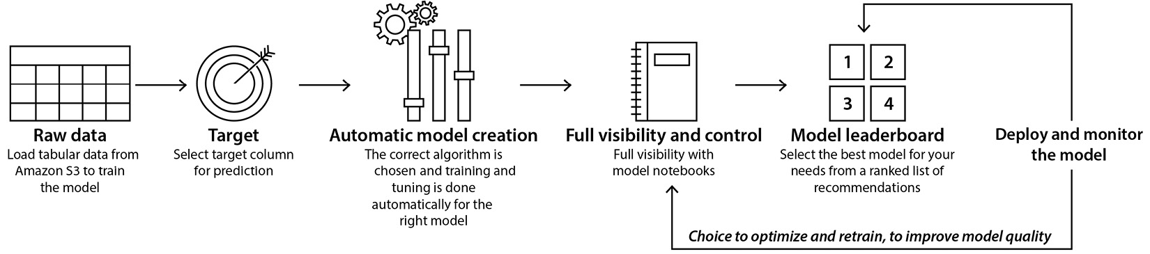
Figure 6.6 – The Azure AutoML Autopilot pipeline

In this section, we introduced AutoML and briefly touched on various AutoML platforms. While each service has its own unique workflow and user experience, they all begin with the same two steps – activating an API and transferring data into a storage repository, or bucket. Following the launch of an experiment run, models can be exported locally or deployed immediately.

The primary distinction between the frameworks lies in the method of entry – web-based, via the command line, or using an SDK. Now that we have covered AutoML, we will move on to the next step, MLOps, the automation process of building models and then deploying and managing them.

The need for MLOps

The journey from AI research to production is long and full of hurdles. The complete AI/ML workload, whether building models, deploying models, or allocating web resources, is cumbersome, as any change in one step leads to changes in another. Even with advancements in deep learning, the process of taking an idea to production can be pretty lengthy.

Figure 6.7 shows the different components of an ML system. We can see that only a small fraction of an ML system is involved in the actual learning and prediction; however, it requires the support of a vast and complex infrastructure. The problem is aggravated by the fact that Changing Anything Changes Everything (CACE), such that minorly tweaking the hyperparameters, changing the learning settings, or modifying the data selection methods can mean that the whole system needs to change:

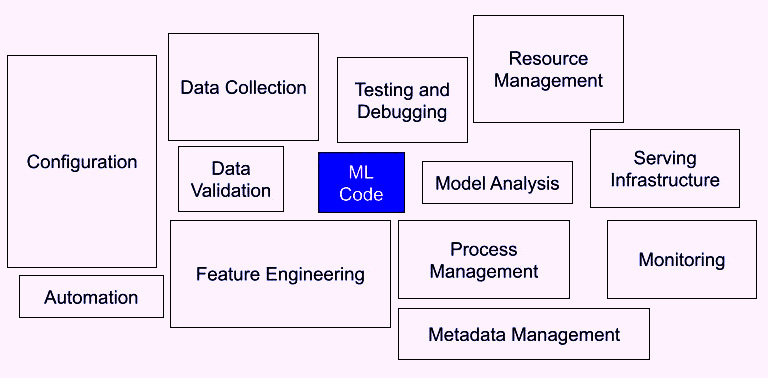
Figure 6.7 – The different components of an ML system

In the IT sector, speed, reliability, and access to information are the main ingredients of success and, hence, provide a competitive advantage. IT agility is required regardless of the remit of an organization. This becomes indispensable when AI/ML-based solutions and products are considered. Currently, most industries play out ML tasks manually, with huge delays between building an ML model and its deployment. This is shown in Figure 6.8:

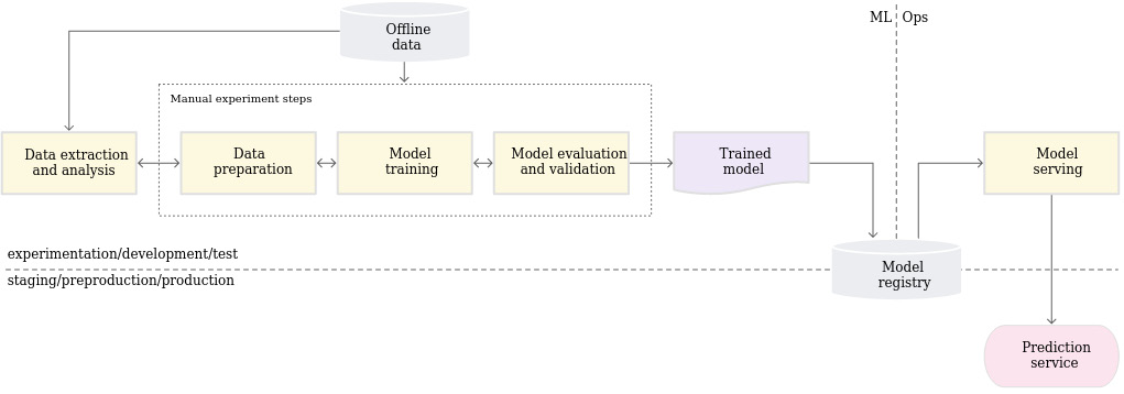
Figure 6.8 – An ML product life cycle (image source: Figure 2: https://cloud.google.com/architecture/mlops-continuous-delivery-and-automation-pipelines-in-machine-learning)

The data collected is prepared and processed (with normalization, feature engineering, and so on) to provide input to the ML model. Model training followed by model evaluation over numerous metrics and techniques is sent to the model registry, where it is containerized to be served.

From data analysis to model serving, each task is conducted manually. Moreover, the transition from one task to another is also manual. The data scientist works independently of the Ops team; the trained model is handed to the development team, who then deploy the model within their API infrastructure. This can bring about training-serving skew – that is, a discrepancy between the model’s performance during training and its performance when it is deployed (served).

As model development is separate from its final deployment, there are infrequent release iterations. Moreover, an immense setback is the scarcity of active performance monitoring. The prediction service does not track or maintain a log of the model predictions necessary to detect any degradation or drift in the behavior of the model and its performance. Theoretically, this manual process could be sufficient if the model were rarely changed or trained. However, in practice, models often fail when they are deployed in the real world. The failure is manifold:

Model degradation: The model’s accuracy drops with time. In the traditional ML pipeline, no continuous monitoring is done to recognize a drop in the model’s performance to redress it. The end user bears the brunt of this. Imagine you provide services to a fashion house that recommends new apparel designs based on the past purchases of customers and fashion trends. However, style changes emphatically with time; the “in” colors in autumn no longer work in winter. If your model does not ingest recent fashion data and utilize it to give customers recommendations, they will complain, and eventually, the site’s user base will shrink. Eventually, the business team will notice, and much later, upon distinguishing the issue, you will be approached to update the model as per the latest data. This situation can be avoided if there is an option to monitor the model’s performance continuously, and the systems in place to implement continuous training for newly acquired data. This is shown in Figure 6.9:

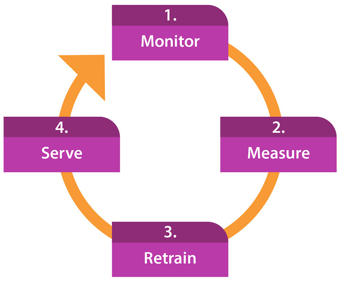
Figure 6.9 – Continuous training

Data drift: The difference between the joint distribution of the input features and the output for training and test datasets can cause dataset drift. When a model is initially deployed, the real-world data has a similar distribution to the training dataset, but this distribution tends to change with time. For instance, you build a model to detect network intrusion based on the data available at that time. After six months, do you think it will work as proficiently as it did at the time of deployment? It may, but chances are it will be fast drifting away – in the rapidly changing internet world, six months is almost six generations! This problem can be resolved if there are options to slice metrics on recent data.
Feedback loops: Unintentional feedback can manipulate a model’s prediction and sway its training data. Suppose somebody works for a music streaming company in which a recommendation system is utilized to suggest new music albums based on a user’s listening history and profile. The system recommends albums with, let’s say, more than a 70% confidence level. Now, the company has decided to add a like or dislike feature. Initially, the company will be excited, as the recommended albums will receive increasing likes. However, over time, the user’s viewing history will impact the model’s predictions. As a result, the system will start recommending music similar to what the user has previously listened to, potentially missing out on new music that the user may enjoy discovering. Continuous system metric monitoring is a potential solution to issues such as this.

To learn more about the technical debt incurred by ML models, I suggest you read the paper titled Machine Learning: The High-Interest Credit Card of Technical Debt by Sculley et al. In this paper, a detailed discussion of the technical debt in ML is carried out, and the maintenance costs associated with systems using AI/ML solutions are also covered.

Although it is impossible and unnecessary to obliterate technical debt completely, a holistic approach can reduce it. What is needed is a system that permits us to integrate standard DevOps pipelines into our ML workflows – ML pipeline automation, or MLOps.

MLOps, or DevOps for ML, is a bunch of best practices that consolidate software development (Dev) and operations (Ops) to speed up the delivery of ML models and prediction-as-a-service apps. The primary objective of MLOps is to improve the quality and speed of model development, deployment, and management while mitigating the perils associated with deployment, making it a salient tool to gain a competitive edge in the market.

Close collaboration between data scientists and engineers is mandatory when it comes to deploying ML models to production. MLOps thus helps automate an ML workflow and caters to end-to-end tracing, from data preparation to model training and from prediction to serving. It also makes ML models reproducible and auditable, which is essential for compliance with regulatory requirements such as the GDPR. MLOps can be difficult to implement, but there are plenty of tools and frameworks that can help, such as Jenkins for Continuous Integration (CI), Spinnaker for Continuous Delivery (CD), and Kubeflow for ML model management. Many open source tools that can be leveraged to create an MLOps pipeline are also up for grabs. Beyond choosing the right tools, culture and collaboration are equally important for implementing MLOps. A successful, cross-functional MLOps team is required. A clear comprehension of the business goals and how ML can assist in accomplishing them should also be considered. Ultimately, MLOps is about moving faster while maintaining high quality and compliance. When done correctly, it can assist businesses in acquiring the upper hand by speeding up ML models and application delivery.

Let’s consider the different ML model life cycle steps (refer to Figure 6.8). Each of these steps can be completed manually or via an automatic pipeline. The level of automation of these steps determines the time gap between training new models and their deployment and, thus, can help solve the problems discussed in the previous section. The automated ML pipeline should be able to do the following:

Allow different teams involved in product development to work independently: Ideally, many teams are involved in an AI/ML workflow, moving from data collection, data ingestion, and model development to model deployment. As discussed in the The need for MLOps section, any change one of the teams makes affects everything else (CACE). An ideal ML pipeline automation should allow teams to work independently on various components without any interference from others.
Actively monitor the model in production: Building the model is not the real challenge. The real challenge resides in maintaining the model’s accuracy in production. This is possible if the model in production is actively monitored, with logs maintained and triggers generated if the model’s performance falls below a certain threshold. This allows you to detect any degradation in performance. This can be done by carrying out online model validation.
Accommodating data drift: The model should evolve with new data patterns that emerge when new data comes in. This can be accomplished by adding an automated data validation step to the production pipeline. Any skew in data schema (missing features or unexpected values for features) should trigger the investigation of the data science team. Any substantial change in the data’s statistical properties should trigger retraining the model.
Continuous Training (CT): In the field of AI/ML, new model architectures appear every week, and you may be keen to experiment with the latest model or tweak your hyperparameters. The automated pipeline should allow for CT. It also becomes necessary when a production model falls below its performance threshold, or a substantial data drift is noticed.
Reproducibility: Additionally, reproducibility is a major issue in AI, to such an extent that NeurIPS, the premier AI conference, has established a reproducibility chair. The aim for researchers is to submit a reproducibility checklist, empowering others to reproduce the results. Modularized components allow teams to work independently and make changes without impacting other teams. This allows teams to narrow down issues to a given component and, thus, helps with reproducibility.
CI/CD: For an expeditious and dependable update at the production level, there should be a robust CI/CD system. Delivering AI/ML solutions rapidly, reliably, and securely can improve your organization’s performance.
Testing: Finally, you may want to perform A/B testing before applying a model to live traffic; this can be accomplished by configuring the new model to serve 10–20% of live traffic. If the new model performs better, he engineer/developer can serve all the traffic; otherwise, roll back to the old model.

In essence, we need MLOps as an integrated engineering solution that unifies ML system development and ML system operation. This will allow data scientists to explore various model architectures, experiment with feature engineering techniques and hyperparameters, and push changes automatically to deployment. Figure 6.10 shows the different stages of the ML CI/CD automation pipeline:

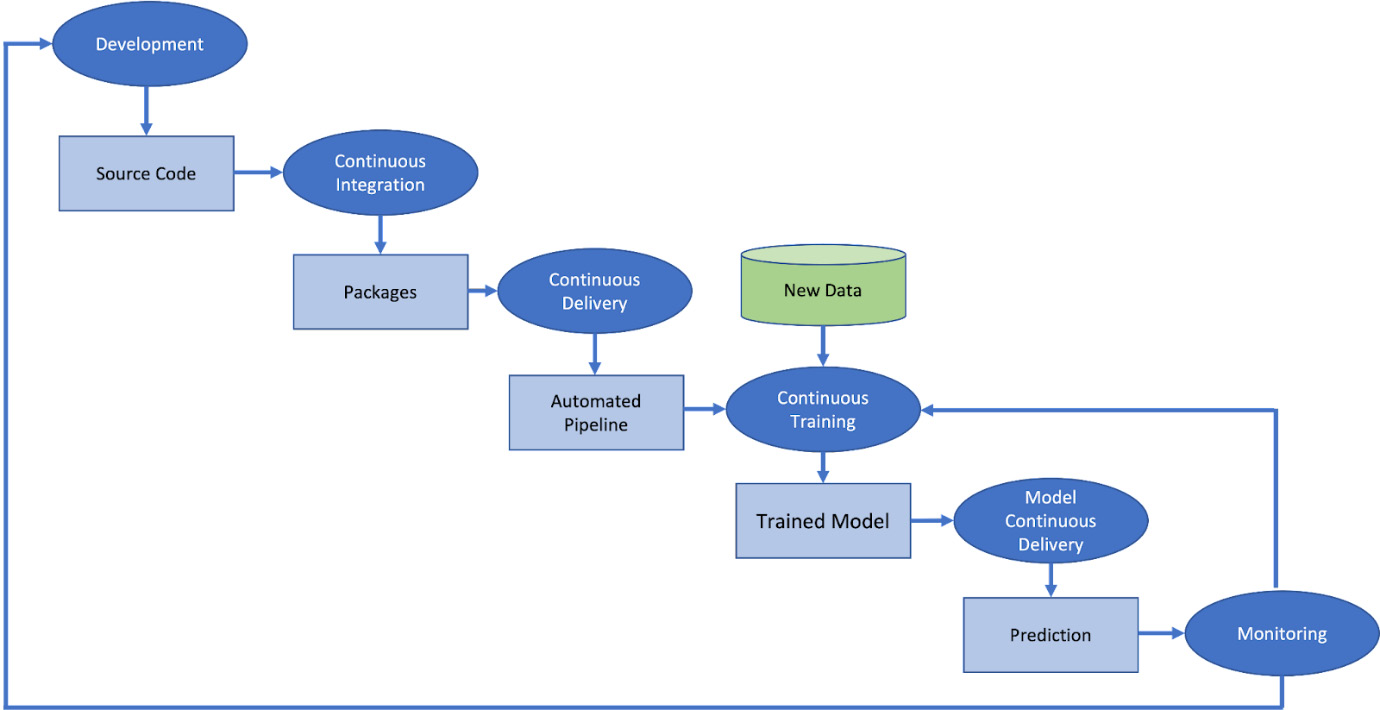
Figure 6.10 – The stages of the automated ML pipeline with CI/CD

The complete automation pipeline comprises six stages:

Development/experimentation: At this stage, the data scientist iteratively tries various ML algorithms and architectures. Once satisfied, they push the model’s source code to the source code repository.
CI of the pipeline: This stage involves building the source code and identifying and outputting the packages, executables, and artifacts that need to be deployed later.
CD of the pipeline: The artifacts produced in stage 2 are deployed to the target environment.
CT: Depending upon the triggers set, a trained model is pushed to the model registry at this stage.
CD of the model: Here, a model prediction service is deployed.
Monitoring: At this stage, the model performance statistics are collected and used to set triggers to execute the pipeline or a new experiment cycle.

In the upcoming sections, we will cover some GCP (short for Google Cloud Platform) tools you can use to implement MLOps. We will talk about Cloud Run, TensorFlow Extended, and Kubeflow, the latter of which is the focus of the chapter (along with Vertex AI).

TFX – a scalable end-to-end platform for AI/ML workflows

TensorFlow Extended (TFX) is a scalable end-to-end platform for creating and deploying TensorFlow AI/ML workflows. TFX comprises libraries for data validation, data pre-processing, feature engineering, AI/ML model creation and training, model performance evaluation, and finally, providing models as REST and gRPC APIs. You can measure the worth of TFX by the fact that it powers several Google products, such as Chrome, Google Search, and Gmail. Google, Airbnb, PayPal, and Twitter all use TFX. As a platform, TFX employs a number of libraries for creating an end-to-end ML process.

Let’s see these libraries and what they can do:

TensorFlow Data Validation (TFDV): This library includes modules for exploring and validating your data. It lets you see the data used to train and/or test a model. The statistical summary provided by it can be utilized to discover any anomalies in the data. It includes an automatic schema creation tool describing the expected data range. It can also be used to detect data drift when comparing various experiments and runs.
TensorFlow Transform (TFT): You can pre-process your data at scale using TFT. The TFT library’s functions can be used to evaluate data, transform data, and conduct advanced feature engineering activities. The use of TFT has the advantage of modularizing the pre-processing procedure. A combination of TensorFlow and Apache Beam allows you to process the full dataset – such as getting the maximum and minimum values or all the available categories – and convert the data batch into tensors. It takes advantage of Google Dataflow, a cloud service.
TensorFlow Estimator and Keras: This is the standard TensorFlow framework you can use to design and train your models. It also gives you access to a large number of pre-trained models.
TensorFlow Model Analysis (TFMA): This enables you to evaluate your trained model, in a distributed manner, on massive volumes of data, using the same model evaluation metrics you established while training. It allows you to analyze and comprehend trained models.
TensorFlow Serving (TFServing): Finally, after you’re happy with your trained model, you can deliver it via REST and gRPC APIs for online production.

The figure here shows how the different libraries are integrated to form a TFX-based AI/ML pipeline:

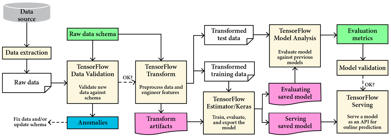
Figure 6.11 – A TFX-based AI/ML pipeline (image source: Figure 4: https://cloud.google.com/architecture/mlops-continuous-delivery-and-automation-pipelines-in-machine-learning)

Each of these stages can be performed manually; however, as mentioned in the preceding section on MLOps, it is preferable for these procedures to be performed automatically. To accomplish this, we require an orchestration tool that connects the various blocks (components) of the ML workflow – this is where Kubeflow comes into play, which will be the topic of the next section.

Understanding Kubeflow

You can manage the full AI/ML life cycle with Kubeflow. It is a native Kubernetes Operations Support System (OSS) platform for developing, deploying, and managing scalable, end-to-end ML workloads in hybrid and multi-cloud settings. Kubeflow Pipelines, a Kubeflow service, aids in the automation of a complete AI/ML life cycle, allowing you to compose, orchestrate, and automate your AI/ML workloads.

It is an open source project, and the following diagram of the commits shows that it is an active and growing project. One of Kubeflow’s key goals is to make it simple for anybody to design, implement, and manage portable, scalable ML. At the time of writing, the Kubeflow GitHub project had 121,000 stars and over 2,000 forks (https://github.com/kubeflow/kubeflow/graphs/contributors):

Figure 6.12 – Contributions to the Kubeflow GitHub repo

The best thing is that you can use the Kubeflow API to design your AI/ML workflow even if you don’t know much about Kubernetes. Kubeflow can be used on your local PC and any cloud (such as GCP or Azure AWS) with a single node or cluster specified; it is designed to work reliably across different settings. Google released Kubeflow 1.2 in November 2022, allowing organizations to operate their ML process across environments. Kubeflow is based on the following three fundamental principles:

Composability: Kubeflow expands Kubernetes’ capacity to perform separate and adjustable tasks by utilizing ML-specific frameworks (such as TensorFlow, PyTorch, and others) and libraries (scikit-learn and pandas). This gives you distinct libraries for different tasks in an AI/ML workflow. Different TensorFlow versions, for example, may be necessary for data preparation and testing. Each job in an AI/ML process may, therefore, be independently containerized and worked upon.
Portability: You can execute all of your AI/ML workflow components from anywhere you want – in the cloud, on-premises, or on your laptop while on vacation – as long as they are all running on Kubeflow.
Scalability: You can use more resources when you wish to and then release them when they are no longer required. Kubeflow increases Kubernetes’ ability to maximize resource availability and scale resources with minimal manual effort.

Some advantages of using Kubeflow are as follows:

It is standardized on a common infrastructure.
It uses open source, cloud-native ecosystems to create, orchestrate, deploy, and run scalable and portable AI/ML workloads across an AI/ML life cycle.
It runs AI/ML workflows in hybrid and multi-cloud environments.
In addition, when running on GKE (short for Google Kubernetes Engine), you can take advantage of GKE’s enterprise-grade security, logging, autoscaling, and identifying features.

Kubeflow populates clusters with Custom Resource Definitions (CRDs). It makes use of containers and Kubernetes. Therefore, it can be used everywhere Kubernetes is already in use.

The Kubeflow applications and components listed here can be used to organize your AI/ML workflow on top of Kubernetes:

Jupyter notebooks: Jupyter notebooks are the de facto tool for quick data analysis for AI/ML practitioners. The majority of data science projects begin with a Jupyter notebook. They serve as the foundation for the contemporary, cloud-native ML pipeline. Kubeflow notebooks allow you to execute your experiments locally, or you can take the data, train the model, and serve it all within a notebook. Notebooks work nicely with the rest of the architecture to provide access to other services in the Kubeflow cluster through the cluster IP addresses. They are also compatible with access control and authentication. Kubeflow allows you to set up several notebook servers, each of which can run multiple notebooks. Depending on a server’s project or team, each notebook server belongs to a specific namespace. Kubeflow supports many users through namespaces, making cooperating and controlling access easier. Using a notebook on Kubeflow allows you to scale resources dynamically. The best part is that it includes all of the plugins/dependencies you’ll need to train a model in Jupyter, including TensorBoard visualizations and customizable compute resources. Kubeflow Notebooks offers the same experience as Jupyter notebooks locally but with the added benefits of scalability, access control, collaboration, and direct job submission to the Kubernetes cluster.
Kubeflow User Interface (UI): A UI for running pipelines, creating and starting experiments, exploring your pipeline’s graph, configuration, and output, and even scheduling runs.
Katib: The tuning of hyperparameters is an important step in the AI/ML workflow. Finding the correct hyperparameter space can be time-consuming. Katib facilitates hyperparameter tuning, early halting, and NAS. It aids in determining the best configuration for production based on the metrics of choice.
Kubeflow Pipelines: Kubeflow Pipelines enables you to create a series of stages that include everything from data collection to providing a trained model. Because they are based on containers, each phase is portable and scalable. Kubeflow Pipelines can be used to orchestrate end-to-end ML workflows. Kubeflow Pipelines takes advantage of the fact that ML operations can be broken down into a series of standard stages that can be placed in the form of a directed graph. Each Kubeflow pipeline job is a self-contained piece of code packaged as a Docker image, complete with inputs (arguments) and outputs. This job containerization enables portability, since the pipelines are self-contained programs that can be run anywhere. Furthermore, the same code can be utilized in another AI/ML pipeline – tasks can be reused.
Metadata: It is helpful to keep track of and manage the metadata that is produced in AI/ML workflows. Tracking metadata can be utilized to perform real-time model evaluation. It can aid in the detection of data drift or training-serving skews. It can also be used for auditing and compliance, allowing you to see which models are in production and how they perform. The metadata component is installed with Kubeflow by default. Many Kubeflow components write to the metadata server. In addition, you can write to the metadata server using your code. The Kubeflow UI can be used to view the metadata – through the artifact store.
KFServing: This allows you to serve AI/ML models on arbitrary frameworks. It includes features such as auto-scaling, networking, and canary rollouts. It has an easy-to-use interface to serve models to production. Using a YAML file, you can provision the resources to serve and compute a model and its prediction. Canary rollouts enable you to test and update models without impacting the user experience.
Fairing: This is a Python package that allows you to build, train, and deploy your AI/ML models in hybrid cloud environments.

To summarize, Kubeflow provides a curated set of compatible tools and artifacts that lie at the heart of running production-enabled AI/ML apps. This helps organizations to standardize a uniform modeling infrastructure across an ML life cycle. Another important step in an AI/ML workflow is hyperparameter tuning, so next, we will explore Katib, which Kubernetes cluster and provides options for both hyperparameter tuning and NAS.

Katib for hyperparameter tuning

Katib is a scalable, Kubernetes-native AutoML platform that facilitates both hyperparameter tuning and NAS. Figure 6.13 shows the design of Katib. To learn more about how it works, readers should refer to Katib: A Distributed General AutoML Platform on Kubernetes:

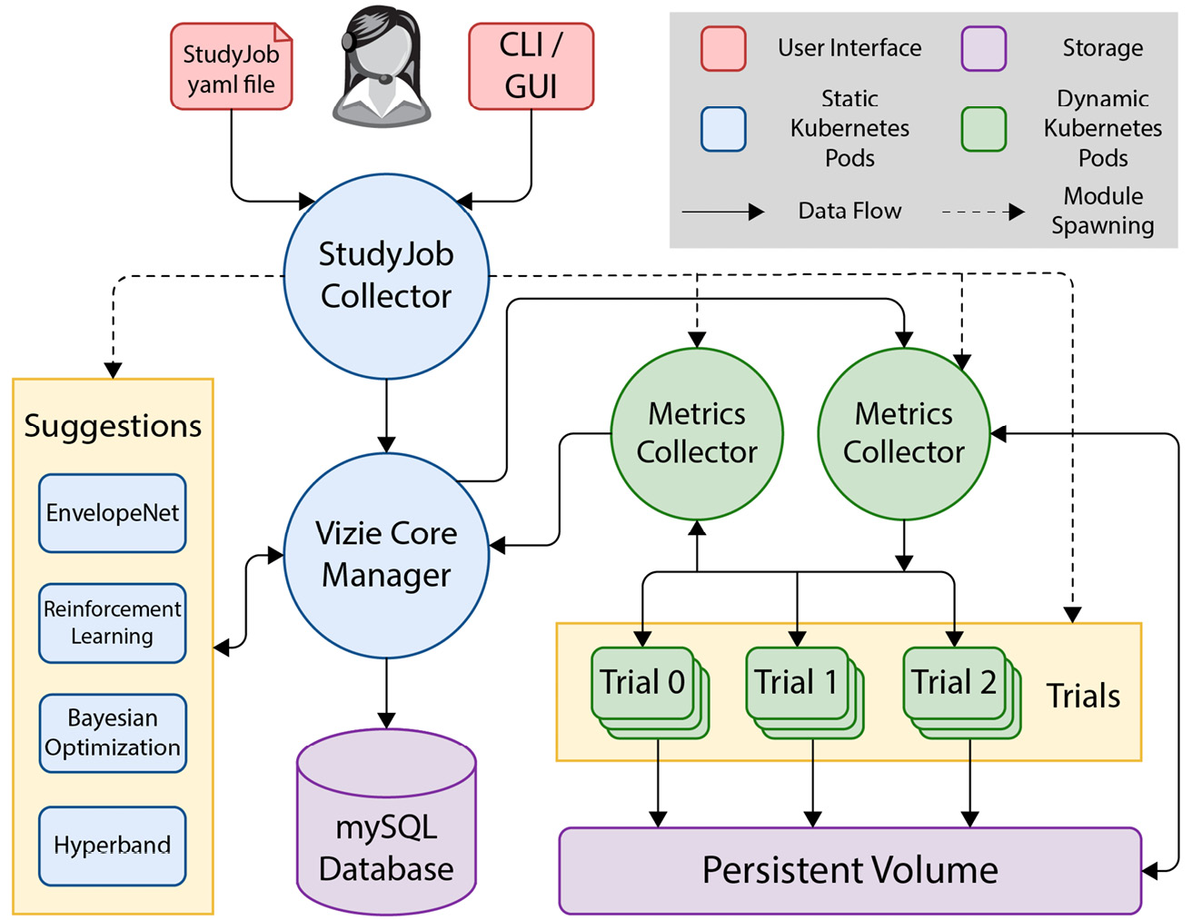
Figure 6.13 – The design of Katib as a general AutoML system (Figure 2 from the paper: https://www.usenix.org/system/files/opml19papers-zhou.pdf)

Katib supports hyperparameter adjustment through the command line via a YAML file specification, as well as the Jupyter Notebook and the Python SDK. It also has a graphical UI for specifying tuning settings and visualizing the results, as shown here:

Figure 6.14 – The graphical interface of Katib

Katib allows you to choose a measure and whether to reduce or increase it. You can choose the hyperparameters you want to tweak and see the results of the entire experiment and individual runs.

Figure 6.15 depicts the outcome of a Katib run, with validation accuracy as the metric and the learning rate, layer count, and optimizer as the hyperparameters to be tuned:

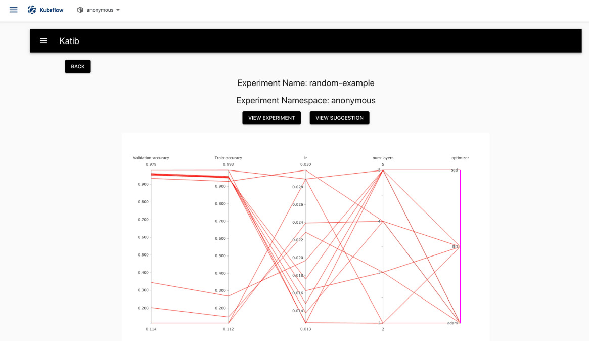
Figure 6.15 – The results of hyperparameter tuning generated by Katib

Another interesting platform for both MLOps and AutoML is Vertex AI, offered by Google, which we will cover next.

Vertex AI

Kubeflow allows you to orchestrate the MLOPs workflow. However, you still need to deal with the Kubernetes cluster. A far better solution would be to not need to worry about the management of clusters at all – enter Vertex AI pipelines. You can use Kubeflow Pipelines or TFX pipelines in Vertex AI. Vertex AI provides tools for every step of the ML workflow, from managing datasets to different ways of training the model, evaluating and deploying it, and making predictions. In short, Vertex AI provides a soup-to-nuts solution for your AI needs. Whether you are a beginner with no code experience but have a great idea that could utilize AI, or you are a seasoned AI engineer, Vertex AI brings something to the table for you. Vertex AI’s AutoML feature makes it easy for beginners to get started with ML; all you have to do is load your data, use the data exploration tools that Vertex AI provides, and start training a model.

Expert AI engineers can create their own training loops, cloud-train their models, and use endpoints to put them into production. Additionally, Vertex AI allows you to do local model training, deployment, and monitoring. Vertex AI is an all-in-one AI/ML platform that features a streamlined UI, as shown in Figure 6.16:

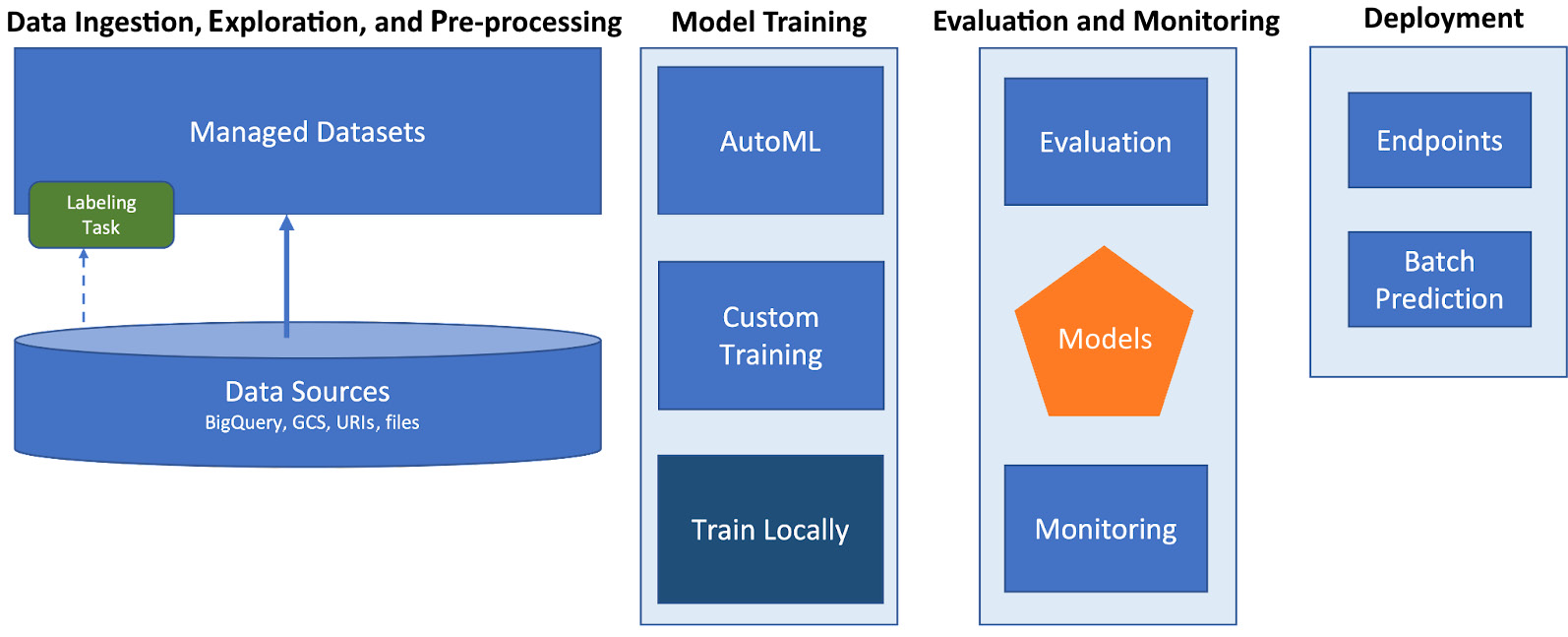
Figure 6.16 – Vertex AI’s unified interface for the complete AI/ML workflow

The Vertex AI dashboard is depicted in Figure 6.17; in the following sections, we will examine its many useful features:

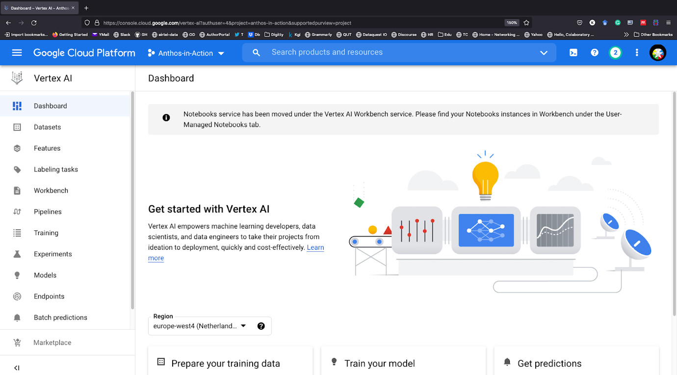
Figure 6.17 – Vertex AI dashboard

Next, we will explore what type of data is supported by Vertex AI and how to handle it.

Datasets

Images, videos, text, and tables are all supported by Vertex AI. You can see a breakdown of the AI/ML tasks that can be completed with Vertex AI-managed datasets in the following table:

Type of data	Tasks supported
Image	Image classification (single-label) Image classification (multi-label) Image object detection Image segmentation
Video	Video action recognition Video classification Video object tracking
Text	Text classification (single-label) Text classification (multi-label) Text entity extraction Text sentiment analysis
Tabular	Regression Classification Forecasting

Table 6.1 – The types of data and types of AI tasks supported on each in Vertex AI

For image, video, and text datasets, if you do not have labels, you can use the annotation service provided by Google. Files containing image URIs and labels can also be imported from your computer. Moreover, you can import data from Google Cloud Storage. It is important to remember that uploaded data will use Google Cloud Storage to store the files you upload from your computer. Only comma-separated values (.csv) files are supported by Vertex AI for tabular data. You can upload them from your local machine, a cloud service, or an import from BigQuery.

Vertex AI allows you to browse and analyze data once it has been specified. If the data is not labeled, you can simply browse it in the browser and assign labels. In addition, Vertex AI provides the option of automating or manually performing the test-training validation split. Figure 6.18 depicts an analysis performed on the HR analytics data (https://www.kaggle.com/arashnic/hr-analytics-job-change-of-data-scientists?select=aug_train.csv) using the Vertex AI managed datasets service.

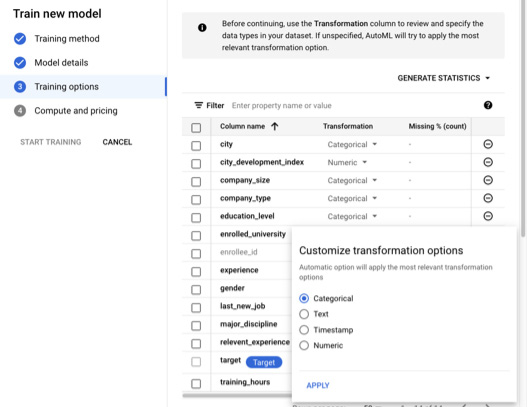
Figure 6.18 – AutoML configurations for tabular data – choosing the training parameters and transformations

Vertex AI also provides a Feature Store option, which can be used to analyze the features of your data. Using the same feature data distribution for training and serving can help reduce training-serving skews. Additionally, Feature Store can help identify model or data drift. In addition, Vertex AI offers a data annotation service for those who need it.

Training and experiments in Vertex AI

The training tasks you have completed and are currently working on are displayed in the Training tab of the Vertex AI dashboard. This can also be the starting point for an entirely new training sequence. Simply select Create and then Create again, and then follow the onscreen prompts to finish the process. You can specify the transformations applied to the tabular data and pick and choose which features to use for training if you choose the AutoML route. The objective function can also be customized. After making your selections, all you have to do is set aside how much time you can afford to train for (the bare minimum is an hour). If the model’s performance isn’t improving during training, it’s best to stop it early, as depicted in Figure 6.19.

The Experiments tab lets you track, visualize, and compare ML experiments and share them with others:

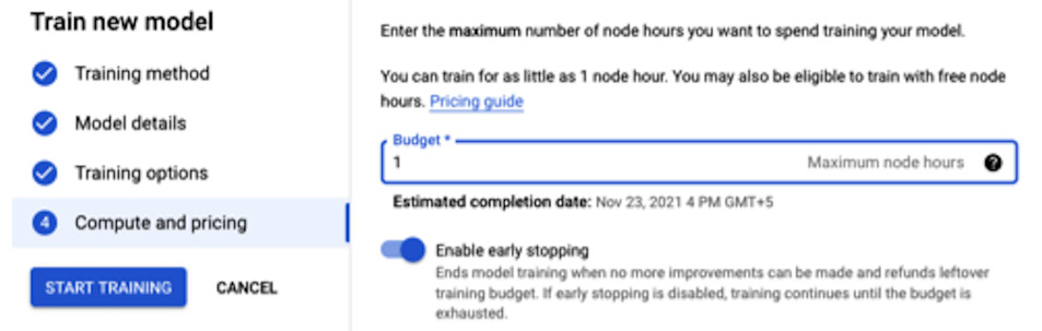
Figure 6.19 – AutoML configurations for tabular data – selecting a budget and early stopping

We have demonstrated Vertex AI AutoML using HR analytics data (https://www.kaggle.com/arashnic/hr-analytics-job-change-of-data-scientists?select=aug_train.csv) to foresee a data scientist’s intention to switch jobs. When training the model, we used everything we had available except the enrolled ID. There is a column in the data files that indicates whether the data scientist is actively seeking employment, and we use this as the target column.

Models and endpoints in Vertex AI

The Models tab contains comprehensive information regarding trained models. These models are complete with a test dataset evaluation (when trained using managed datasets). Additionally, feature importance for all features can be accessed in the case of tabular data. The data can be viewed visually or read as text directly on the dashboard.

The training of models was allotted a 1-node-per-hour budget. The total duration of the training was about 1 hour and 35 minutes. The AutoML-trained model’s test-dataset evaluation is displayed in Figure 6.20:

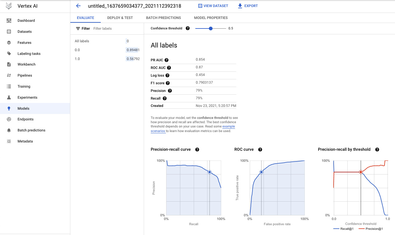
Figure 6.20 – The model evaluation for the test dataset

Now refer to the following figure, which shows the matrix and feature importance:

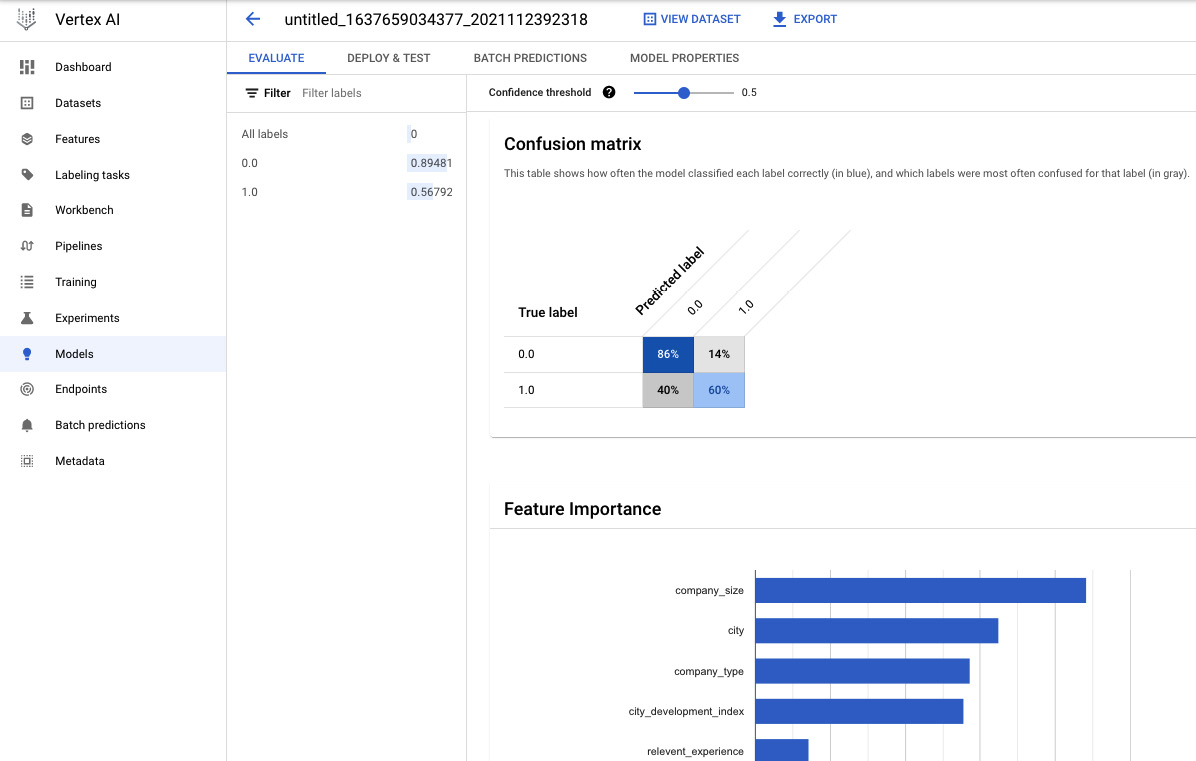
Figure 6.21 – The confusion matrix and feature importance

The dashboard makes it easy to examine a model’s forecast. For testing purposes, the model must be deployed to an endpoint. Vertex AI also provides the option to save the model in a container (in the TensorFlow SavedModel format), which can then be used to launch the model in any other on-premises or cloud service. Let’s go ahead and select Deploy to Endpoint to send the model somewhere. The following choices are available for deployment:

Give a name to the endpoint.
Choose the traffic split – for a single model, it is 100%, but if you have more than one model, you can split the traffic.
Choose the minimum number of compute nodes.
Select the machine type.
Vertex AI provides a sampled Shapley explainability method for tabular data if you choose the model explainability option.
Select which aspects of the model you wish to keep an eye on (feature drift or training-serving skews) and adjust your alert settings accordingly.

Deployment is quick and easy after the initial setup is complete. Let’s now put the prediction to the test (both individual and batch predictions are available). It is clear from Figure 6.22 that the data scientist is not actively seeking employment at a confidence level of approximately 0.67, given the inputs that were chosen. We can use either a REST API or a Python client to send a test request to the model. The Vertex AI endpoint provides the relevant code to accommodate both sample requests.

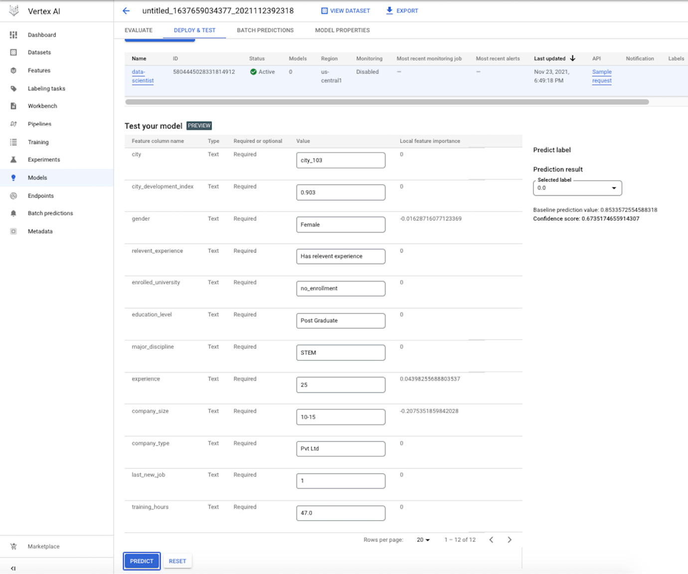
Figure 6.22 – The model prediction

All the models and endpoints deployed in the project are listed in the Models and Endpoints tabs on the dashboard respectively.

Vertex AI Workbench

Vertex AI Workbench is compatible with JupyterLab and the Jupyter Notebook. A user can choose between pre-made notebooks and managed notebooks. All the popular deep learning frameworks and modules are included in managed notebooks, and you can even add your own Jupyter kernels using Docker images. The user-managed notebooks provide a number of useful starting points. Users can configure their notebooks with a choice of virtual central processing units (vCPUs) and graphics processing units (GPUs). If you’re new to Vertex AI and want to get started right away, we recommend starting with the managed notebooks. However, if you’re looking for more administrative power, user-managed notebooks are the way to go.

In order to enter your JupyterLab environment after a notebook has been made, click on the OPEN JUPYTERLAB link.

Figure 6.23 – A list of Jupyter notebooks in Vertex AI Workbench

Vertex AI Workbench can be used in conjunction with TFX or Kubeflow to perform data exploration, model construction, and training and execute code.

Vertex AI provides a unified interface for all the AI/ML process components. You can set up pipelines for model training and experimentation. The interface provides a simple method to tweak hyperparameters. Custom training can be selected, allowing a user to choose from containers and load their code straight away to train on their chosen machine. Vertex AI also features AutoML integration to accelerate the ML workflow. Using AutoML, you can obtain an efficient ML model for controlled datasets with minimal ML skills. Using feature attribution, Vertex AI also provides explainability for its models. When your model is complete, you can select endpoints for batch or single predictions and deploy your model to them. The most important aspect of deployment is the ability to deploy on edge devices and place your model where the data is.

Summary

This chapter provided a comprehensive overview of AutoML and MLOps. It began by introducing the concept of AutoML and explained how it is used to automate the process of training and tuning a large selection of candidate models. The chapter also included a hands-on example of using H2O AutoML and discussed the AutoML features provided by Microsoft Azure and Amazon SageMaker Autopilot. Following that, the chapter introduced the concept of MLOps and the importance of incorporating it into AI/ML workflows.

The chapter covered the features of TFX briefly, which is a TensorFlow-based toolkit to build a full-fledged ML pipeline. It provides a set of libraries and pre-built components that can be used to build and deploy ML models easily.

Kubeflow, an open source project that aims to make running ML workloads on Kubernetes simple, portable, and scalable, was also covered. We also showed how to perform hyperparameter tuning using Katib, which is a Kubernetes-based system for hyperparameter tuning.

Finally, Google’s Vertex AI was explored. This platform provides a simple and easy-to-use interface to build, deploy, and manage ML models. Using Vertex AI, we trained and deployed a model trained on HR analytics data.

Now that you are familiar with the ML pipeline and the various tools used to automate it, in the next chapter, we will move on to the concept of fairness in data collection.

Ética, Direito e Inteligência Artificial Hyperparameter Tuning, MLOps, and AutoML

Ética, Direito e Inteligência Artificial

Hyperparameter Tuning, MLOps, and AutoML

Technical requirements

Introduction to AutoML

Introducing H2O AutoML

Understanding Amazon SageMaker Autopilot

The need for MLOps

TFX – a scalable end-to-end platform for AI/ML workflows

Understanding Kubeflow

Katib for hyperparameter tuning

Vertex AI

Datasets

Training and experiments in Vertex AI

Vertex AI Workbench

Summary

Further reading