The Ethics of Model Adaptability

This chapter gives a detailed overview of detecting different types of model drift for model governance purposes in organizations. The primary objective of this chapter is to demonstrate variations of ML models, with multiple examples to give you an awareness of the importance of the different statistical measures available for detecting data changes and model metric variations. This will help data scientists and MLOps professionals to choose the right drift detection mechanisms and stick to the correct model metric performance thresholds to control risks arising due to incorrect predictions. You’ll learn how to quantify and explain model drift and answer questions related to the need for model calibration. This will also allow you to understand the scope of designing fairly calibrated models.

In this chapter, these topics will be covered in the following sections:

Adaptability framework for data and model drift
How we can explain ML models when subjected to drift or calibration
Understanding the need for model calibration

Technical requirements

This chapter requires you to have Python 3.8 and to run the following commands before starting:

pip install alibi-detect
pip install river
pip install detecta
pip install nannyml (dependency numpy==1.21.0)
git clone https://github.com/zelros/cinnamon.git
python3 setup.py install
git clone https://github.com/Western-OC2-Lab/PWPAE-Concept-Drift-Detection-and-Adaptation.git

The alibi-detect package mentioned in the installation step can be found on GitHub. For reference, you can check out more details of the project at https://github.com/SeldonIO/alibi-detect.

Adaptability framework for data and model drift

Data processing depends on the way data is accessed based on its availability, whether it’s sequential or continuous. Along with the data processing and modeling techniques built on different modes of incoming data, various factors (internal and external) cause the data distribution to change dynamically. This change is called concept drift, and it creates several threats to ML models in production. In concept drift terminology, and as far as the shift in data distributions is concerned, the term window is used to refer to the most recently known concept that was used to train the current or most recent predictor.

Examples of concept drift can be seen in e-commerce systems where ML algorithms profile the shopping patterns of the user and provide personalized recommendations of relevant products. Factors that result in concept drift include events such as marriage and relocating to a different geographical region. The COVID-19 pandemic caused a drastic change in consumers’ buying behavior, because people were forced to turn to e-commerce platforms for online shopping. This resulted in higher demand for products than expected, causing a high rate of prediction errors in forecasting demand in supply chain networks. The e-commerce, supply chain, and banking industries have experienced changes in incoming data patterns, leading to model drift.

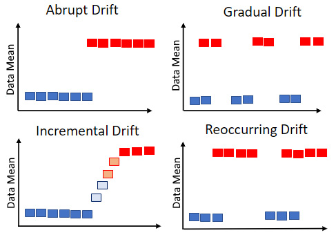
Figure 11.1 – Four types of concept drift

As illustrated in Figure 11.1, there are four kinds of concept drift, caused by various internal or external factors, or even adversarial activities:

Abrupt: Caused by behavior shifts
Incremental: A sudden change with slower decay
Reoccurring: Similar to seasonal trends
Gradual: Slow, long-lasting changes

Other indirect factors, such as the speed of learning, errors in reporting the right features (or units of measurement), and large changes in the classification or prediction accuracy, can also result in concept drift. This is illustrated in Figure 11.2. To address concept drift, we need to update the models causing the drift. This could be a blind update or training with weighted data, model ensembling, an incremental model update, or applying modes of online learning.

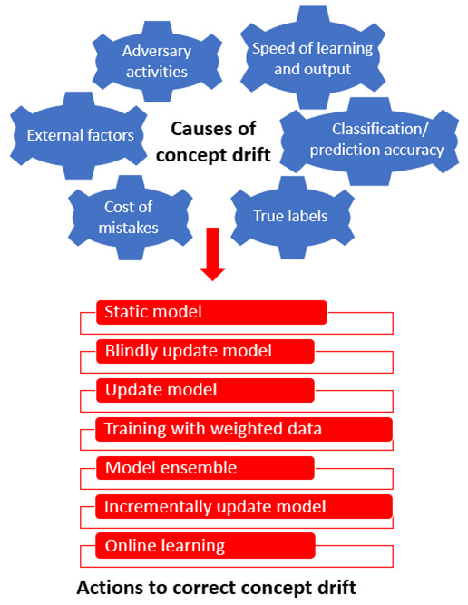
Figure 11.2 – Different types of drift-causing factors and remedial actions

We categorize concept drift detectors (illustrated in Figure 11.3) primarily based on the batch or online data arrival mode. Batch detection techniques can further be classified into whole-batch and partial-batch detection techniques. The size and sample of the batch are two of the factors used to classify them as whole-batch or partial-batch detection. Online detectors are further classified based on their ability to manipulate the reference window in order to detect drift. The detection window is often a sliding window that moves with an incoming instance, often referred to as the current concept. However, fixed reference windows are also used to detect concept drift.

Online detectors function by evaluating the test statistics computed for the first W data points and then updating the test statistics. The updates can be done sequentially at a lower cost, thereby helping us to detect fluctuations in the test statistics beyond a threshold value. A value exceeding the threshold indicates that drift has taken place.

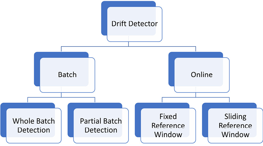
Figure 11.3 – Commonly used drift detectors

Figure 11.3 illustrates the idea of unsupervised batch-based (with a fixed window) and online-based (fixed and sliding windows) drift detection techniques that, after necessary data distribution comparison and a significance test, detect whether there has been drift or not. Batch-based methods may require instance selection and statistical computations on a batch to confirm the testing of drift conditions, enabling us to infer whether drift has occurred or not. The numbers here signify the sequence of steps required to detect both online and offline drift.

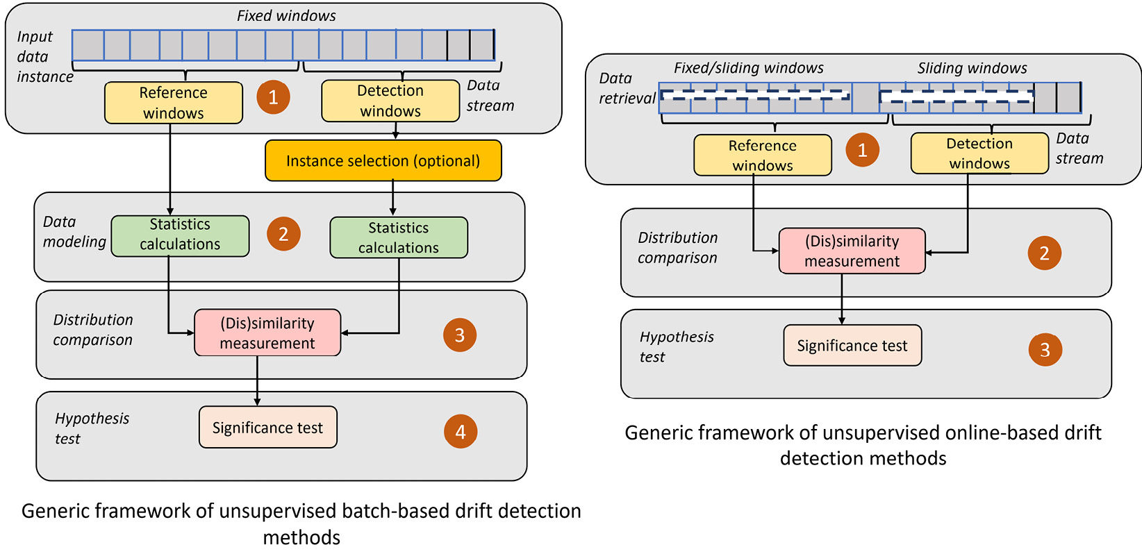
Figure 11.4 – Online and batch drift detection methods

An example of an online drift adaptive framework is the Performance Weighted Probability Averaging Ensemble (PWPAE) framework, which can be used effectively in IoT anomaly detection use cases.

This framework can be deployed on IoT cloud servers to process big data streams using a wireless medium from IoT devices. This kind of ensemble adaptive drift detector is composed of four base learners that help with real-time drift detection:

An Adaptive Random Forest (ARF) model with an ADWIN drift detector (referred to as ARF-ADWIN)
An ARF model with a DDM drift detector (referred to as ARF-DDM)
A Streaming Random Patches (SRP) model with an ADWIN drift detector (referred to as SRP-ADWIN)
An SRP model with a DDM drift detector (referred to as SRP-DDM)

The four base online learners are combined by weighting them based on their accuracy and classification probabilities. Let’s try the PWPAE framework on the CICIDS2017 (https://www.unb.ca/cic/datasets/ids-2017.html) simulated intrusion detection dataset, which contains benign and recent common attacks, resembling true real-world examples:

To run PWPAE, let’s first make the necessary imports from the river package:

from river import metrics
from river import stream
from river import tree,neighbors,naive_bayes,ensemble,linear_model
from river.drift import DDM, ADWIN

Then we set up the PWPAE model with X_train and y_train to train the model, and we test it on X_test and y_test. The following code snippet uses the PWPAE model:
```
name = "Proposed PWPAE model"
t, m = PWPAE(X_train, y_train, X_test, y_test)
acc_fig(t, m, name)
```

The trained results and the comparative outputs are visualized in Figure 11.5.

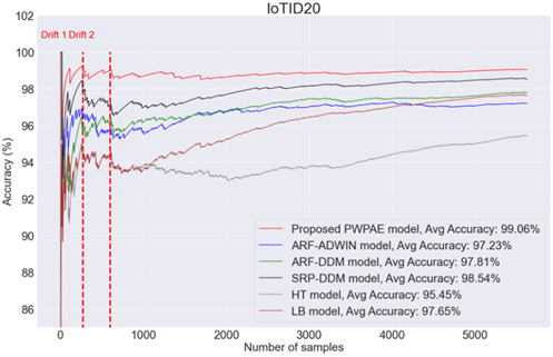
Figure 11.5 – The performance results of PWPAE with the Hoeffding Tree (HT) and Leveraging Bagging (LB) models

The accuracy of PWPAE is 99.06% and it exceeds the accuracy of other models.

Let us investigate some supervised drift detection strategies where actual feedback for prediction is available and is used with the predicted outcomes to yield error metrics.

Statistical methods

Statistical methods help us to compare and assess two different distributions. A divergence factor or a distance metric can be used to measure the difference between two distributions at different points in time to understand their behavior. This helps with the timely detection of the model’s performance metrics and finding the features that are causing the change.

Kullback–Leibler divergence

Kullback–Leibler (KL) divergence, also popularly known as relative entropy, quantifies how much one probability distribution differs from another. Mathematically, it can be stated as follows:

Q is the distribution of the old data and P is the distribution of the new data for which we compute the divergence, and || represents the divergence. When P(x) is high and Q(x) is low, the divergence will be high. On the other hand, if P(x) is low and Q(x) is high, the divergence will be high but not too high. When P(x) and Q(x) are similar, then the divergence will be low. The following code creates a KL divergence plot for a (P, Q, M) distribution with a mean of 5 and a standard deviation of 4:

x = np.arange(-10, 10, 0.001)
q = norm.pdf(x, 5, 4)
plt.title('KL(P||Q) = %1.3f' % kl_divergence(p, q))
plt.plot(x, p)
plt.plot(x, q, c='red')

The change in distribution patterns due to KL divergence is illustrated in Figure 11.6:

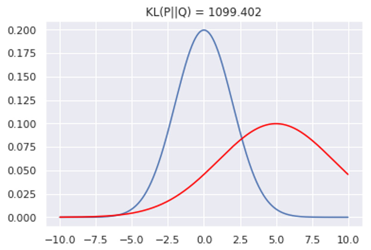
Figure 11.6 – KL divergence

There are more forms of divergence, which we will look at next.

Jensen–Shannon divergence

Jensen–Shannon (JS) divergence uses KL divergence and can be formulated mathematically as follows:

One difference between KL and JS divergence is that JS divergence is symmetrical with a mandatory finite value. The change in distribution patterns due to JS divergence is illustrated in Figure 11.7:

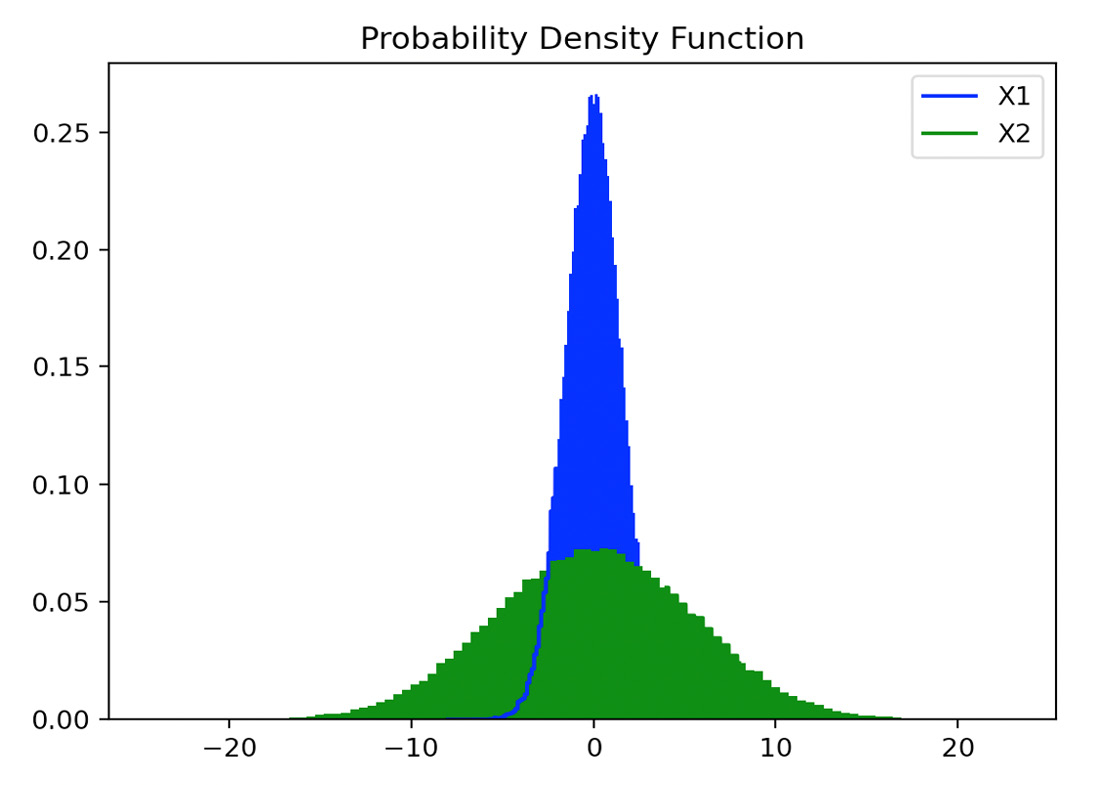
Figure 11.7 – JS divergence

To compute JS and KL divergence, we run the following code snippet:

First, we create a normal distribution for distribution 1:

data1 = scipy.stats.norm.rvs(size=100000, loc=0, scale=1.5, random_state=123)
hist1 = np.histogram(data1, bins=100)
hist1_dist = scipy.stats.rv_histogram(hist1)
import matplotlib.pyplot as plt
X1 = np.linspace(-8.0, -2.0, 1000)
plt.title("PDF")
plt.hist(data1, density=True, bins=100,  color ='blue')
plt.plot(X1, hist1_dist.pdf(X1), label='PDF', color = 'blue')

Next, we create another normal distribution, which is our second distribution:

data2 = scipy.stats.norm.rvs(size=100000, loc=0, scale=5.5, random_state=123)
hist2 = np.histogram(data2, bins=100)
hist2_dist = scipy.stats.rv_histogram(hist2)
X2 = np.linspace(4.0, 8.0, 1000)
plt.title("Probability Density Function")
plt.hist(data2, density=True, bins=100, color ='green')
plt.plot(X2, hist2_dist.pdf(X2), label='PDF', color = 'green')
plt.legend(['X1', 'X2'])

In the next step, we first evaluate the KL divergence between probability distribution 1 and the mean of the two Probability Density Functions (PDFs) of Y1 and Y2 and the same for probability distribution 2:
```
Y1 = hist1_dist.pdf(X1)
Y2 = hist2_dist.pdf(X2)
M = (Y1 + Y2) / 2
d1 = scipy.stats.entropy(Y1, M, base=2)
print("KL div Y1 and M", d1)
d2 = scipy.stats.entropy(Y2, M, base=2)
print("KL div Y2 and M", d2)
```

The previous step yields the following output:

KL div X1 and X2 0.21658815880427068
KL div Y1 and M 1.0684247605300703
KL div Y2 and M 0.1571132219534354

In the next step, we first evaluate the JS divergence between the distributions and also within each distribution individually:
```
js_dv = (d1 + d2) / 2
js_distance = np.sqrt(js_dv)
print("JS Dist d1 and d2", js_distance)
```

We evaluate this against the SciPy calculation of JS divergence between the distributions:

js_distance_scipy = scipy.spatial.distance.jensenshannon(Y1, Y2)
print("JS Dist d1 and d2 of Scipy", js_distance_scipy)
js_distance_scipy = scipy.spatial.distance.jensenshannon(X1, X2)
print("JS Dist X1 and X2 of Scipy", js_distance_scipy)
dx1 = scipy.stats.entropy(Y1, X1, base=2)
dx2 = scipy.stats.entropy(Y2, X2, base=2)
js_dv = (dx1 + dx2) / 2
print("JS Div X1 and X2", js_dv)

The preceding step yields the following output:

JS Dist d1 and d2 0.7827956254615587
JS Dist d1 and d2 of Scipy 0.6037262820103958
JS Dist X1 and X2 of Scipy 0.1941318696014193
JS Div X1 and X2 1.3749093686870903

The first distance gives the symmetric JS divergence, while the second evaluated metric gives the JS distance, which is the square root of the JS divergence. The third and fourth distance metrics evaluated give us the JS distance between X1, X2 and dx1, dx2, respectively. dx1 and dx2 here signify the entropy of distributions created from Y1, X1 and Y2, X2, respectively.

The Kolmogorov-Smirnov test

The two-sample Kolmogorov-Smirnov (KS) test is a general nonparametric method used to differentiate two samples. The data change pattern, best identified by the KS test, is illustrated in Figure 11.8. The Cumulative Distribution Function (CDF) of (sample, x) quantifies the percentage of observations below x on the sample. This can be obtained by doing the following:

Sorting the sample
Counting whether the number of observations within the sample is less than or equal to x
Dividing the numerator computed in step 2 by the total number of observations on the sample

The purpose of the drift detector is to detect drift patterns when two distribution functions observe a change, causing a shape change in two samples:

Figure 11.8 – KS test

Population stability index

Population stability index (PSI) is a metric that monitors and measures shifts in population behavior between two samples or over two periods of time. It serves as a risk-scorecard metric to give a probable risk estimation between an out-of-time validation sample and a modeling sample including both dependent and independent variables. The application of PSI can also be extended to compare the education, income, and health status of two or more populations in social-demographic studies.

Model distillation is a technique that allows the transfer of knowledge from a large network to a small network, which trains a second model with a simplified architecture on soft targets (the output distributions or the logits) retrieved from the original model. It paves the way to detect adversarial and malicious data and data drift by comparing the output distributions of both the original model and the distilled model.

Let us now see, with an example, how adversarial scores are detected by the model distillation detector in the context of drift detection. The KS test has been used as the scoring function to run a simple univariate test between the adversarial scores of the reference batch and the test data. A high adversarial score indicates a harmful drift, and a flag is raised for malicious data drift. Here, we can fetch the pretrained model distillation detector from a Google Cloud bucket or train one from scratch:

First, we import the necessary packages from alibi_detect:

from alibi_detect.cd import KSDrift
from alibi_detect.ad import ModelDistillation
from alibi_detect.models.tensorflow.resnet import scale_by_instance
from alibi_detect.utils.fetching import fetch_tf_model, fetch_detector
from alibi_detect.utils.tensorflow.prediction import predict_batch
from alibi_detect.utils.saving import save_detector
from alibi_detect.datasets import fetch_cifar10c, corruption_types_cifar10c

Then, we define and train the distilled model:

from tensorflow.keras.layers import Conv2D, Dense, Flatten, InputLayer
from tensorflow.keras.regularizers import l1
def distilled_model_cifar10(clf, nb_conv_layers=8, distl_model_filters1=256, nb_dense=40, kernel1=8, kernel2=8, kernel3=8, ae_arch=False):
    distl_model_filters1 = int(distl_model_filters1)
    distl_model_filters2 = int(distl_model_filters1 / 2)
    distl_model_filters3 = int(distl_model_filters1 / 4)
    layers = [InputLayer(input_shape=(64, 64, 3)),
              Conv2D(distl_model_filters1, kernel1, strides=2, padding='same')]
    if nb_conv_layers > 2:
        layers.append(Conv2D(distl_model_filters2,
kernel2, strides=2, padding='same', activation=tf.nn.relu, kernel_regularizer=l1(1e-5)))
    if nb_conv_layers > 2:
        layers.append(Conv2D(distl_model_filters3, kernel3, strides=2, padding='same',
                             activation=tf.nn.relu, kernel_regularizer=l1(1e-5)))
    layers.append(Flatten())
    layers.append(Dense(nb_dense))
    layers.append(Dense(clf.output_shape[1], activation='softmax'))
    distilled_model = tf.keras.Sequential(layers)
    return distilled_model

Next, based on our configuration, we can either load a pretrained model or train a new model:

load_pretrained = True
detector_type = 'adversarial'
detector_name = 'model_distillation'
filepath = os.path.join(filepath, detector_name)
if load_pretrained:
    ad = fetch_detector(filepath, detector_type, dataset, detector_name, model=model)
else:
    distilled_model = distilled_model_cifar10(clf)
    print(distilled_model.summary())
    ad = ModelDistillation(distilled_model=distilled_model, model=clf)
    ad.fit(X_train, epochs=50, batch_size=128, verbose=True)
    save_detector(ad, filepath)

We now plot the mean scores and standard deviations per severity level. We define the model accuracy plot as the mean and standard deviation of the harmfulness and no-harmfulness scores:

def evaluate_plot_model_accuracy():
mu_noharm, std_noharm = [], []
mu_harm, std_harm = [], []
acc = [clf_accuracy['original']]
for k, v in score_drift.items():
   mu_noharm.append(v['noharm'].mean())
   std_noharm.append(v['noharm'].std())
   mu_harm.append(v['harm'].mean())
   std_harm.append(v['harm'].std())
   acc.append(v['acc'])

The plot (illustrated in Figure 11.9) shows the mean harmfulness scores (the line plot starting from the left-hand side) and ResNet-32 accuracies (the bars displayed on the right-hand side) for increasing data corruption severity levels. Level 0 corresponds to the original test set. We have demonstrated the impact of varying levels of malicious (corrupted) data along with its severity levels.

Harmful scores signify instances that gave an incorrect prediction because of corrupted data. Even not-harmful predictions are known to exist, which remains unchanged (as shown by the harmful index, marked in yellow along the Y axis) after the data corruption due to the injection of malicious adversarial samples. To summarize further, we see in Figure 11.9 that the corruption severity increases as the harmfulness score increases (shown by the cyan bars) and the accuracy decreases (shown by the blue line).

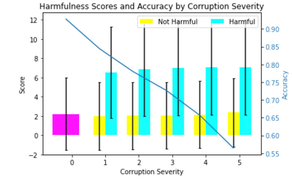
Figure 11.9 – Distilled drift detector detecting the corruption severity

There are some other methods that we can categorize as contextual methods.

Contextual methods

The purpose of these methods is to compare and assess the difference between the train and test datasets and evaluate the drift when there’s a significant difference in the predicted outcomes.

Tree features

This method enables you to train a simple tree based on data and prediction timestamps that are fed as independent input features, along with other features. Once the tree model is analyzed for feature importance, it is evident that the effect on data at different points in time helps to substantiate the differences arising due to concept drift. The tree splits, and the feature splits done on the timestamp, help to explain the changes due to drift.

Shuffling and resampling (SR)

The data is split into train and test sets at an assumed drift point, and then the model is trained using the train dataset and evaluated against the test dataset to compute the error rates. The same mechanism of training and testing is repeated by shuffling the same dataset and recomputing the error metrics. Drift is said to be detected when the difference between the ordered data error rate and the average shuffled data error rate is above a specified threshold. This is also a computationally intensive mechanism as it involves training multiple models during occurrences of drift.

Statistical process control

This kind of drift detector control mechanism ensures that when the model in production generates varying accuracy metrics over time, the errors in the model can be managed. Though this method is effective in detecting sudden, gradual, and incremental drift in a short span of time, the latency could be high when extracting labels from the samples. The requirement of having labeled data makes it more difficult to be applied widely.

Drift detection method (DDM)

This method of drift detection is one of the earliest devised. Incoming data is assumed to be in a sequence following a binomial distribution and a Bernoulli trial variable (or single data point) inferring the occurrence of drift based on the prediction error rate.

The algorithm records the minimum probability of error (p) rate and the minimum standard deviation (s) of the binomial distribution when p + s reaches its own minimum. Drift is said to be present when the p + s value exceeds the sum of the minimum probability of error (pmin) and a multiple of the minimum standard deviation (smin). We can state that as (p + s) > (pmin + 3 ✶ smin).

The recommended multiplying factor is 3. This method has limitations when the change occurs slowly, where the cache/memory may overflow.

Early Drift Detection Method (EDDM)

This method, although similar to DDM, focuses on gradual drift by computing the mean (m) and standard deviation (s) of the distance between two errors. It records (m + 2 ✶ s) and when it reaches its maximum value, it saves both values as mmax and smax , respectively. When the ratio, (m + 2 ✶ s)/(m + 2 ✶ smax), drops below a threshold (β; the recommended value is 0.9), drift is detected, and an alarm should be raised.

CUSUM and Page-Hinkley

Cumulative Sum (CUSUM) and its variant, Page-Hinkley (PH), both rely on a sequential analysis technique, typically from an average Gaussian signal. These methods detect the change and raise an alarm when they observe that the difference between the observed values and the mean is higher than a user-defined threshold. As the changes are sensitive to the parameter values, one disadvantage of this is the triggering of false alarms. These methods can be widely applied to data streams.

CUSUM

This drift detection algorithm detects small changes in the mean using CUSUM. When the probability distributions before and after the change are known, then the CUSUM procedure optimizes an objective function by considering the delays and frequency of false alarms. It has the additional advantage of being simple and intuitive to interpret in terms of maximum likelihood. It is memoryless, one-sided, and asymmetrical, with the ability to detect only an increase in the difference between the observed value and the mean.

The CUSUM detector is a kernel-based technique that continuously compares samples from the database. The metric for drift determination is called the Maximum Mean Discrepancy (MMD). This procedure is well suited for large data volumes because it does not need to compare pre- and post-distributions, instead concentrating on the current data to identify drift. CUSUM has been enhanced to use a dual mean value on nested sliding windows, which is called the Double CUSUM Based on Data Stream (DCUSUM-DS). Another variant of CUSUM is DCUSUM-DS, which uses a dual mean value CUSUM. The DCUSUM-DS algorithm works on nested sliding windows and detects drift by calculating the average value of the data within the window twice. After detecting the average, it extracts new features and then generates accumulated and controlled graphs to avoid false inference. One major benefit of this method is that it can detect new features and rerun its analysis to ensure it detects the correct drift and does not rely only on the average values detected.

The kernel-based variant of CUSUM does not require the pre- and post-change distributions and instead depends on a database of samples from the pre-change distribution, with which it can continuously compare incoming observations with samples from the database. The kernel function chosen by the user and the statistical metric for comparison is MMD. The Kernel Cumulative Sum (KCUSUM) algorithm works well in settings where there is a huge amount of background data available, and when it is necessary to detect deviations from the background data.

The algorithm can be configured with a threshold that sets the limit beyond which an alarm is triggered. The magnitude of the drift threshold (say, 80%, 50%, or 30%) helps us to obtain the right metric for identifying a drift. Accordingly, an alarm needs to be raised when any deviations in the data or model pattern are observed. For example, an algorithm can be set to a very large amplitude with an 80% threshold boundary, which will enable it to detect drift more frequently than when it is set to 30%. The detector returns the following values:

ta: Change detection index – a return value that represents the alarm time (the index when the change was detected)
tai: Starting index of change – shows the index when the change started
taf: Ending index of change – denotes the index when the change ended (if ending is True)
amp: Denotes the amplitude of the changes (if ending is True)

One way to configure the parameters is to start with a very large threshold value and set drift to half of the expected change. We can also adjust drift so that g is 0 more than 50% of the time. We can then fine-tune threshold so the required number of false alarms or delays in detecting drift is obtained. For faster drift detection, we need to decrease drift, whereas to reduce false alarms and minimize the effect of small changes, we need to increase drift.

The following code snippet demonstrates how to use the CUSUM drift detector:

from detecta import detect_cusum
x = np.random.randn(500)/5
x[200:300] += np.arange(0, 4, 4/100)
ta, tai, taf, amp = detect_cusum(x, 4, .025, True, True)
x = np.random.randn(500)
x[200:300] += 6
detect_cusum(x, 3, 1.5, True, True)
x = 2*np.sin(2*np.pi*np.arange(0, 2.8, .01))
ta, tai, taf, amp = detect_cusum(x, 1.8, .05, True, True)

The preceding code is able to detect drift between a range of data, illustrated in the following figure, by drift percentage, threshold, and the number of instances of change.

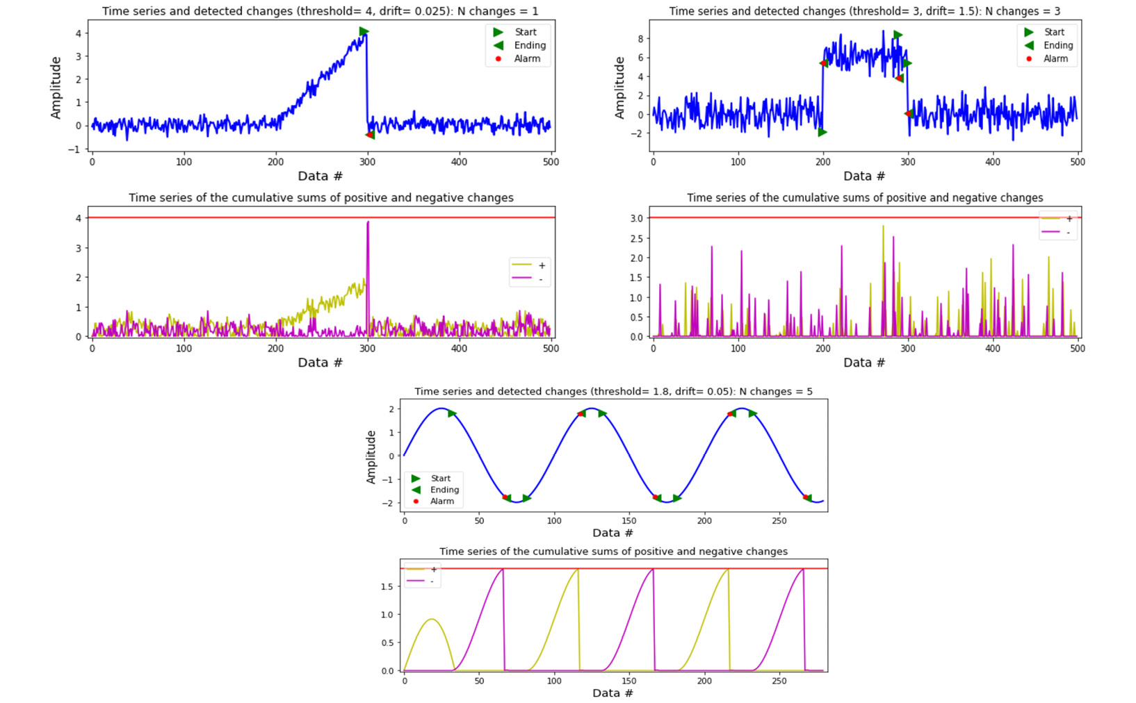
Figure 11.10 – CUSUM drift detector change detections

The threshold-based drift detection technique used here demonstrates (Figure 11.10) the role of the CUSUM of positive and negative changes in detecting drift.

Covariate and prior probability data drift

Covariate drift occurs due to changes in the distributions of one or more of the independent features due to internal or external factors, but the relationship between the input X and target Y remains the same. While the distribution of input feature X changes with covariate data drift, with prior probability shift, the distribution of the input variables remains the same but the distribution of the target variable changes. Changes in the target distribution result in prior probability data drift. To implement covariate drift, we apply a shift to the mean of one of the normal distributions.

The model is now being tested on a new region of the feature space, causing the model to misclassify new test observations. In the absence of true test labels, it is impossible to measure the model’s accuracy. Here, the drift detector helps by detecting whether covariate or prior probability drift is occurring. If it’s the latter, a proxy for prior drift can be monitored by initializing the detector on labels from the reference set, which is then fed into a model’s predicted labels to identify drift.

The following steps illustrate how to detect data drift by comparing it with the original model trained on the initial dataset:

First, we take a multivariate normal distribution and then specify the reference data to initialize the detectors:

shift_norm_0 = multivariate_normal([2, -4], np.eye(2)*sigma**2)
X_0 = shift_norm_0.rvs(size=int(N_test*phi1),random_state=2)
X_1 = ref_norm_1.rvs(size=int(N_test*phi2),random_state=2)

We stack the reference distributions and try to estimate the drift by comparing it with true_slope, which has been set to -1:

phi1 = phi1*1.5
phi2 = phi2*2.5
true_slope = -1
shift_norm_0 = multivariate_normal([3, -8], np.eye(2)*sigma**2)
X_0 = shift_norm_0.rvs(size=int(N_test*phi1),random_state=2)
X_1 = ref_norm_1.rvs(size=int(N_test*phi2),random_state=2)
X_test = np.vstack([X_0, X_1])
y_test = true_model(X_test,true_slope)
plot(X_test,y_test,true_slope,clf=clf)
print('Mean test accuracy %.2f%%' %(100*clf.score(X_test,y_test)))
pred = detector.predict(X_test)
print('Is drift? %s!' %labels[pred['data']['is_drift']])

The code snippet generates the following plots to demonstrate a use case of no drift versus covariate drift, exhibiting lower mean accuracy where there is drift (right side) than where there is none (left side).

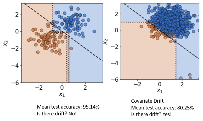
Figure 11.11 – Covariate data drift

While Figure 11.11 shows covariate data drift, the following code demonstrates the use of the MMD method, in which an estimate of the expected squared difference between the kernel conditional mean embeddings of Xref | C and Xtest | C are computed to evaluate the test statistic:
```
def detect_prior_drift():
    label_detector = MMDDrift(y_ref.reshape(-1,1), backend='tensorflow', p_val=.05)
    y_pred = clf.predict(X_test)
    label_detector.predict(y_pred.reshape(-1,1))
detect_prior_drift()
```

We get the following output:

{'data': {'is_drift': 1,
  'distance': 0.107620716,
  'p_val': 0.0,
  'threshold': 0.05,
  'distance_threshold': 0.013342142},
 'meta': {'name': 'MMDDriftTF',
  'detector_type': 'offline',
  'data_type': None,
  'version': '0.9.0',
  'backend': 'tensorflow'}}

The MMD detector detects drift with a distance of 0.1076, and the threshold of drift detection is 0.013342.

Least-squared density difference

The Least-squared density difference (LSDD) drift detection technique directly estimates the density difference without separately estimating the densities of the prior and the current distribution. In the following sample code, the dataset is shuffled and normalized so that each feature takes a value in the range of [0,1] and predicts the same binary outcomes.

The LSDD online drift detector from alibi_detect necessitates an Expected Runtime (ERT) (an inverted False Positive Rate (FPR)), allowing the detector to run an average number of steps in the absence of drift before making a false detection. With a high ERT, detectors lose their sensitivity and become slow to respond, so the configuration adjusts the trade-off between the ERT and the expected detection delay to target desirable ERTs. The best way to simulate the desired configuration is to select training data that is an order of magnitude larger than the desired ERT:

In the following code snippet, the model is trained on white wine samples, which form the reference distribution, and red wine samples are drawn from a drifted distribution. The steps following the upcoming code block illustrate how to run LSDD drift detection, and how it helps to compare no drift versus drift:

white, red = np.asarray(white, np.float32), np.asarray(red, np.float32)
n_white, n_red = white.shape[0], red.shape[0]
col_maxes = white.max(axis=0)
white, red = white / col_maxes, red / col_maxes
white, red = white[np.random.permutation(n_white)], red[np.random.permutation(n_red)]
X = white[:, :-1]
X_corr = red[:, :-1]
X_train = X[:(n_white//2)]
X_ref = X[(n_white//2) :(3*n_white//4)]
X_h0 = X[(3*n_white//4):]
X_ref = np.concatenate([X_train, X_ref], axis=0)

In the first run, without the detector set, we do not detect any drift:

n_runs = 550
times_h0 = [time_run(cd, X_h0, window_size) for _ in range(n_runs)]
print (f"Average run-time under no-drift: {np.mean(times_h0)}")
_ = scipy.stats.probplot(np.array(times_h0), dist=scipy.stats.geom, sparams=1/ert, plot=plt)

The preceding code yields the following output:

Average run-time under no-drift: 47.72

The following code snippet imports LSDDDriftOnline from alibi_detect and sets it up with reference data, ert, window_size, the number of runs, and a TensorFlow backend both for the original and current distributions to detect drift. Then, the online drift detector is run with an ert value of 50 and window_size of 10:

X_new_ref = np.concatenate([X_train, X_ref], axis=0)
from alibi_detect.cd import LSDDDriftOnline
def lsdd_detector():
    cd = LSDDDriftOnline(
        X_new_ref, ert, window_size, backend='tensorflow', n_bootstraps=5500,
    )
 times_h0 = [time_run(cd, X_h0, window_size) for _ in range(n_runs)]
    print(f"Average run-time under no-drift: {np.mean(times_h0)}")
    _ = scipy.stats.probplot(np.array(times_h0), dist=scipy.stats.geom, sparams=1/ert, plot=plt)

This produces the following output:

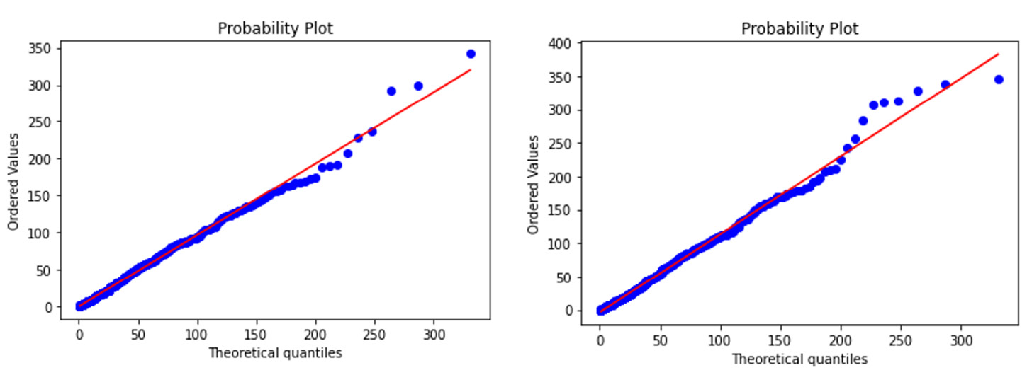
Figure 11.12 – LSDD drift detector

Figure 11.12 demonstrates online drift detection with LSDD. Here, we let the detector run a configurable number of times (50) or iterations and configure 5,500 bootstraps to detect the drift. The bootstraps are used to run the simulations and configure the thresholds. A greater magnitude helps to achieve better accuracy in terms of obtaining the ERT, and it is typically configured to be an order of magnitude larger than the ERT.

We get the following output:

Average run-time under drift: 54.39

Furthermore, we observe that the detector on the held-out reference data in the first run follows a geometric distribution with mean ERT, without having any drift. However, as soon as drift is detected, the detector is very fast to respond, as shown in Figure 11.12.

Page-Hinkley

This method of drift detection functions by detecting changes by computing the observed values and their mean up to the current moment. Without issuing any warning signals, it runs the PH test to detect concept drift if the observed mean is found to exceed a threshold lambda value. Mathematically, it can be formulated as follows:

When gt– Gt > h, an alarm is raised.

Now, let us walk through the step-by-step process of detecting drift using the PH method:

The following code sample demonstrates how we simulate two distributions:

import random
from river import drift
import matplotlib.pyplot as plt
import numpy as np
rng = random.Random(123456)
ph = drift.PageHinkley()

Now, we compose and plot a data stream composed of three data distributions:

data_stream = rng.choices([50, 100], k=1200) + rng.choices(range(600, 900), k=5000) + rng.choices(range(200, 300), k=5000)
plt.plot(data_stream)
plt.show()

Now, we update the drift detector and see whether a change has been detected:

for I, val in enumerate(data_stream):
     in_drift, in_warning = ph.update(val)
     if in_drift:
       print (""Change detected at index {i}, input value: {val"")

We get the following output. We see that drift is detected for three different distributions of the graph at different points in time. The change detection points are printed on two sides of the plot.

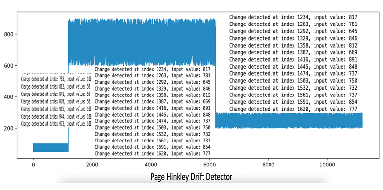
Figure 11.13 – Drift detected at three ranges of a distribution with a PH detector

The Fast Hoeffding Drift Detection Method

The Fast Hoeffding Drift Detection Method (FHDDM) allows the constant tracking of a sliding window of values of the probability of correct predictions along with the maximum observed probability values. A drift is said to have occurred when the correct prediction probability drops below the maximum configured value, along with the difference in probabilities exceeding a threshold.

Paired learner

The paired learner (PL) mechanism includes two learners, one of which is a stable learner that gets trained on all data, and the other learner is trained on recent data. A counter is incremented each time the stable learner makes an error in prediction but the recent learner does not. To account for mistakes, a counter is decremented each time the recent learner makes an error in prediction. Once the increment counter exceeds a specified threshold, drift is considered to have occurred. This mechanism involves heavy computation to train new models and to have two learners in place.

Exponentially Weighted Moving Average Concept Drift Detection

In the Exponentially Weighted Moving Average Concept Drift Detection (ECDD) method, the exponentially weighted moving average (EWMA) forecast is used by calculating the forecast’s mean and standard deviation continuously. It is often used to monitor and detect the misclassification rate of a streaming classifier. Drift is detected when the forecast exceeds the sum of the mean plus a multiple factor/coefficient of the standard deviation.

Feature distribution

This drift detection technique functions without response feedback by identifying a change in p(y|x) due to a corresponding change in p(x). This change can be detected using any multivariate unsupervised drift detection technique.

Drift in a regression model

To detect drift in a regression model, you take the regression error (a real number) and apply any unsupervised drift detection technique to the error data.

Ensemble and hierarchy drift detectors

Ensemble detectors work primarily on an agreed consensus level, where consensus can be derived from only a few, all, or a majority of learners. Hierarchical detectors come into play only after drift is detected by a detector at the first level using any of the drift detection techniques discussed previously. Then, the consensus approach can be used to validate the result at other levels, starting from the next level. Some ensemble and hierarchy drift detector algorithms include Linear Fore Rates (LFR), Selective Detector Ensemble (eDetector), Drift Detection Ensemble (DDE), and Hierarchical Hypothesis Testing (HLFR).

Now that we have looked at different types of concept drift detection techniques, let us discuss model explainability whenever there is drift/calibration.

Multivariate drift detection with PCA

To detect drift from multivariate data distributions, we use Principal Component Analysis (PCA) by compressing the data to a lower-dimensional space and then decompressing the data to retrieve the original feature representation. As we preserve only the relevant information in the transformation process, the reconstruction errors (evaluated using the Euclidean distance between the original and transformed data) help us to identify a change in data relationships among one or multiple features. In the first step, we compute the PCA on the original reference dataset and store the reconstruction errors with allowable limits of upper and lower thresholds. The process is repeated with the new data, where we compress and decompress the data using PCA. When the reconstruction errors exceed the upper or lower threshold, it signifies a change in data distribution.

The following code demonstrates how we can detect multivariate feature drift:

In the first step, we have the necessary imports:

import numpy as np
import pandas as pd
import matplotlib.pyplot as plt
import seaborn as sns
import nannyml as nml
from scipy.spatial.transform import Rotation

Next, we have a random data setup based on its three features:

# analyze with reference and analysis periods
# Days/week * Hours/day * events/hour
DPP = 7*24*24
np.random.seed(23)
s1 = np.random.randn(DPP*22)
x1 = s1 + np.random.randn(DPP*22)/8
x2 = s1 + np.random.randn(DPP*22)/8
x3 = np.random.randn(DPP*22)/8
xdat = np.array([x1, x2, x3]).T
rot = Rotation.from_euler('z', 90, degrees=True)
# following matrix multiplication implementation, we need a 3xN data matrix hence we transpose
ydat = np.matmul(rot.as_matrix(), xdat.T).T
# drift is sudden and affects last 5-7 weeks
dataar = np.concatenate(
(xdat[:-5*DPP], ydat[-5*DPP:]),
axis=0)
datadf = pd.DataFrame(dataar, columns=['feature1', 'feature2', 'feature3'])
datadf = datadf.assign(ordered = pd.date_range(start='1/3/2020', freq='5min', periods=22*DPP))
datadf['week'] = datadf.ordered.dt.isocalendar().week - 1
datadf['partition'] = 'reference'
datadf.loc[datadf.week >= 8, ['partition']] = 'analysis'
datadf = datadf.assign(y_pred_proba = np.random.rand(DPP*22))
datadf = datadf.assign(y_true = np.random.randint(2, size=DPP*22))

Next, we can do a further interpretation of the independent feature, but the goal is to set up the drift detector as follows:

rcerror_calculator = nml.DataReconstructionDriftCalculator(
feature_column_names=feature_column_names,
timestamp_column_name='ordered',
chunk_size=DPP
).fit(reference_data=reference)
rcerror_results = rcerror_calculator.calculate(data=analysis)
figure = rcerror_results.plot(plot_reference=True)
figure.show()

This yields what is shown in Figure 11.14, where we see that the data has drifted from 0.84 to 0.80.

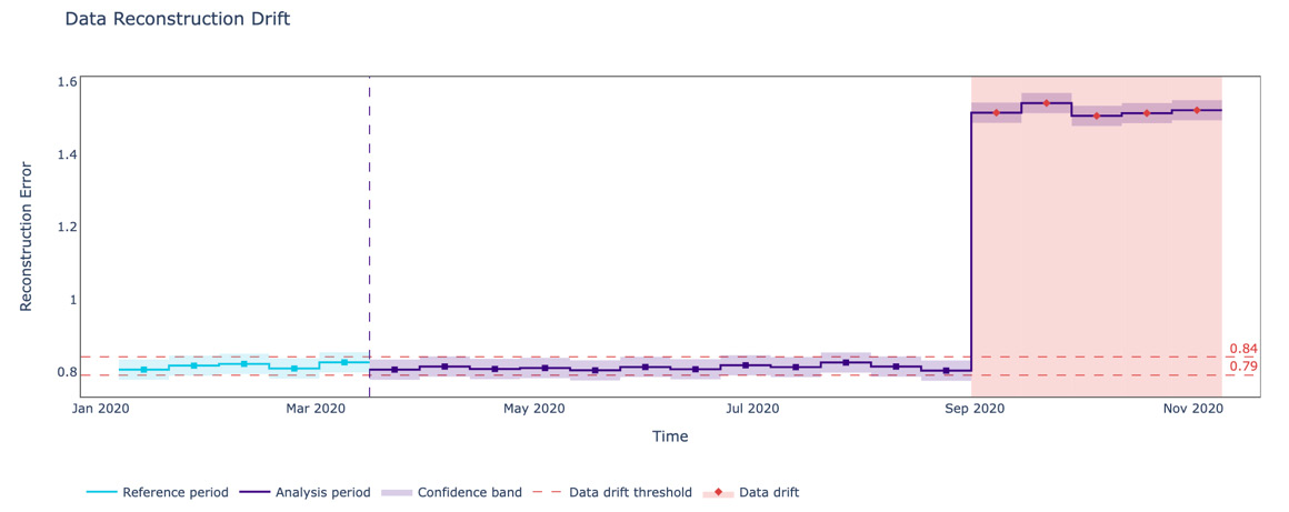
Figure 11.14 – Multivariate drift detector using PCA

Understanding model explainability during concept drift/calibration

In the preceding section, we learned about different types of concept drift. Now, let us study how we can explain them with interpretable ML:

First, we import the necessary packages for creating a regression model and the drift explainer library. The California Housing dataset has been used to explain concept drift:

from xgboost import XGBRegressor
from cinnamon.drift import ModelDriftExplainer, AdversarialDriftExplainer
from sklearn import datasets
from sklearn.datasets import fetch_california_housing
from sklearn.datasets import fetch_openml
california = fetch_openml(name="house_prices", as_frame=True)
california_df = pd.DataFrame(california.data, columns=california.feature_names)
RANDOM_SEED = 2021

Then, we train the XGBoost regressor model:

model = XGBRegressor(n_estimators=1000, booster="gbtree",objective="reg:squarederror", learning_rate=0.05,max_depth=6,seed=RANDOM_SEED, use_label_encoder=False)
model.fit(X=X_train, y=y_train, eval_set=[(X_test, y_test)], early_stopping_rounds=20, verbose=10)

In the next step, we fit our trained model using ModelDriftExplainer, plot the prediction, and retrieve any drift, if it is observed by the explainer:

drift_explainer = ModelDriftExplainer(model)
drift_explainer.fit(X_train, X_test, y_train, y_test)
drift_explainer.plot_prediction_drift()
drift_explainer.get_prediction_drift()

The following figure illustrates differences in drift detection in two different datasets.

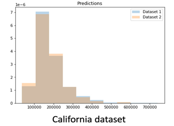
Figure 11.15 – Drift from the input features or data distributions of two datasets

In Figure 11.15, it is evident that there isn’t any apparent drift in the distributions of the predictions.

Then, we plot the target labels to evaluate any drift in the predicted outcomes:
```
drift_explainer.plot_target_drift()
drift_explainer.get_target_drift()
```

However, as shown in Figure 11.16, we do not observe any apparent drift in the target labels:

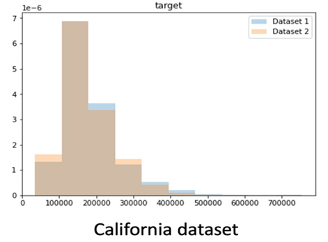
Figure 11.16 – Drift from the target data distributions of the California Housing dataset

In the next step, when we evaluate the performance metrics of the California Housing train and test datasets, we can see a data drift from the mean and the explained variance of the performance metrics:
```
drift_explainer.get_performance_metrics_drift()
```

On running the drift explainer on the California Housing dataset, we get the following output:

PerformanceMetricsDrift(dataset1=RegressionMetrics (mse=10567733.794917172, explained_variance=0.9983637108518892), dataset2=RegressionMetrics(mse=540758766.1766539, explained_variance=0.9088298308495063))

Our next task is to plot drift values computed with the tree-based approach, obtain the feature importances of the California Housing dataset, and use AdversarialDriftExplainer on the datasets. This is illustrated in Figure 11.17, which clearly shows that the Neighborhood_OldTown and BsmtQual_Gd features are the features most impacted by the drift:

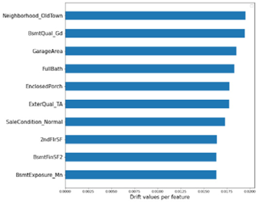
Figure 11.17 – Feature importance in the resultant drift

In the end, we can plot each feature and evaluate the drift for each of them, as shown in Figure 11.18. Here, Neighborhood_OldTown, the first feature, does not show any noticeable drift between the train and test datasets:
```
drift_explainer.plot_feature_drift('Neighborhood_Old_Town')
drift_explainer.get_feature_drift('Neighborhood_Old_Town')'
```

The preceding code snippet yields the following output, showing the difference between the two datasets is not significant, as p_value is 0.996 > 0.05:

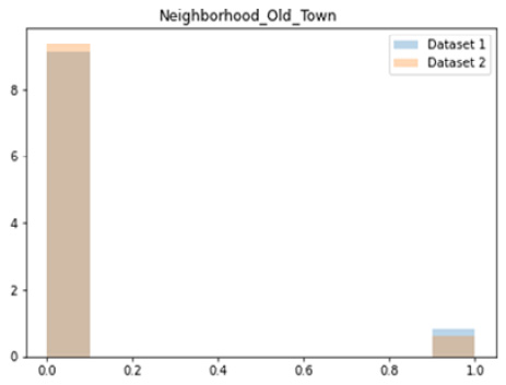
DriftMetricsNum(mean_difference=-0.022504892367906065, wasserstein=0.022504892367906093, ks_test=BaseStatisticalTestResult (statistic=0.022504892367906065, pvalue=0.996919812985332))

Figure 11.18 – Distribution differences/drift due to the Neighborhood_Old_Town feature

After gaining an understanding of drift, as data scientists, we also need to understand when we need to calibrate our models in the event of any change.

Understanding the need for model calibration

Recommendation systems (content-based filtering or hybrid systems) are used in almost all industry sectors, including retail, telecoms, and energy and utilities. Deep learning recommendation models using user-to-user or item-to-item embeddings with explainability features have been able to build trust and confidence and improve the user experience. Deep learning recommendation systems have often used attention distributions to explain the neural network’s performance, but such explanations in the case of natural language processing (NLP) are limited by poor calibrations of deep neural networks.

It has been observed that models become less reliable due to over-confidence or under-confidence impacting models designed for healthcare (disease detection) and autonomous driving, among others. In such a scenario where model reliability comes into question, it is important to have a metric such as model calibration in place so that the degree of a model’s predicted probability is correlated with its true correctness likelihood, which determines the model’s performance.

In other words, a calibrated model can be called authentic when it has a high confidence level (more than 80%, say) where more than 80% of the predictions are classified accurately. We can also use model calibration to plot reliability plots. This serves as the accuracy of the model by interpreting reliability as a function of its confidence in the predictions. An over-confident model’s reliability plot falls below the identity function, while an under-confident plot’s reliability goes above the identity function. We also see that an authentic calibrated model provides the perfect classification boundary where the reliability plot can be benchmarked as the identity function.

Figure 11.19 contains a reliability plot for the Deep Item-Based Collaborative Filtering (DeepICF) model. DeepICF examines nonlinear and higher-order relationships among all interacting item pairs by training them using nonlinear neural networks. It can help us to understand how we model the predictions in different groups and study the trade-off between accuracy and confidence through a reliability plot.

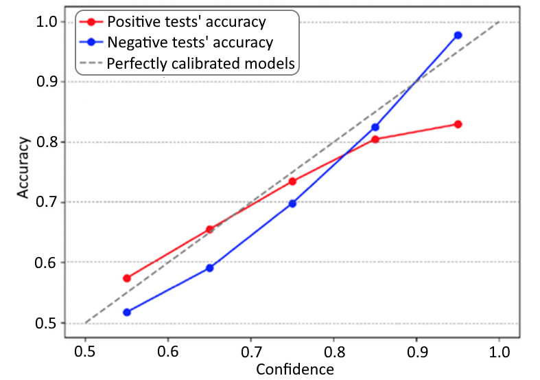
Figure 11.19 – A reliability plot for the DeepICF model

We segmented the model predictions into different buckets based on their confidence and calculated the accuracy for each of them. Figure 11.19 demonstrates the DeepICF model (with attention networks: https://www.researchgate.net/publication/333866071_Model_Explanations_under_Calibration) becoming over-confident as the confidence increases for both positive and negative classes. The DeepICF model is a deep neural network that is produced after learning latent low-dimensional embeddings of users and items. The pair-wise user and item interactions are captured with a neural network layer by means of an element-wise dot product. Further, the model also uses attention based pooling to yield an output vector of fixed size. This leads to a drop in accuracy for imbalanced and negatively skewed datasets, demonstrating that model explanations generated from the attention distribution become less reliable with over-confident predictions.

Now, let us discuss how explainability and model calibration can be brought together when we see drifts in a model’s predicted outcomes.

Explainability and calibration

Model explainability and proper model calibration can be achieved by addressing imbalance in the dataset and by adding stability to attention distributions. However, one more problem that needs to be addressed is the calibration drift resulting from the same factors as concept drift. One example evident in the healthcare industry is poorly calibrated risk predictions with changing patient characteristics and disease incidence or prevalence rates in different health centers, regions, and countries. When an algorithm is trained in a setting with a high disease incidence, it is dominated by the model inputs and yields overestimated risk estimates. When such calibration drift occurs due to the deployment of models in nonstationary environments, these models require retraining and recalibration. Recalibration helps to fix the model’s accuracy and confidence levels and, consequently, the reliability plot.

Now, let us see, with an example, why it is necessary to calibrate a recommendation model, which is most useful in the following situations:

When a change in user preferences is observed due to the addition of new customer segments in the population
When a change in user preferences is observed among existing customers
When there are promotions/campaigns or new products are released

In the following example, let us study how post-preprocessing logic can be embedded in an underlying recommendation algorithm to ensure the recommendation becomes more calibrated. To explain this problem, we will use movielens-20m-dataset:

To compute the utility metrics of recommender systems, we must compute the KL divergence between the user-item interaction distribution and the recommendation distribution. Here, we have chosen an associated lambda term that controls the score and calibration trade-off. The higher the lambda, the higher the probability that the resulting recommendation will be calibrated:
```
def compute_recommendation_utility(reco_items, interacted_distr, lmbda=0.65):
    total_score = 0.0
    reco_distr = compute_likely_genres(items_to_recommend)
    kl_div = evaluate_kl_divergence(interacted_distr, reco_distr)
    for item in items_to_recommend:
        total_score += item.score
    rec_utility = (1 - lmbda) * total_score - lmbda * kl_div
    return rec_utility
```

The utility function defined here is invoked at each iteration to update the list with the item that maximizes the utility function:

def calibrate_recommendations(items, interacted_distr, topn, lmbda=0.65):
    calib_rec_items = []
    for _ in range(topn):
        max_utility = -np.inf
        for rec_item in items:
            if rec_item in calib_rec_items:
                continue
            rec_utility = compute_recommendation_utility(calib_rec_items + [rec_item], interacted_distr, lmbda)
            if rec_utility > max_utility:
                max_utility = rec_utility
                best_item = rec_item
        calib_rec_items.append(best_item)
    return calib_rec_items

The lambda term allows us to tweak the controller (lambda) to extremely elevated levels to generate the modified calibrated recommendation list. Now, let us differentiate and evaluate the computed recommendation generated after calibrating it (to optimize the score, 𝑠), the original recommendation, and the user’s past relationship with the items. Here, 𝑠(𝑖) represents the score of the items, 𝑖∈𝐼, predicted by the recommender system, and s(I) = ∑i ∈ Is(i) denotes the sum of all the items’ scores in the newly generated list:
```
calib_rec_item_distr = compute_likely_genres(calib_items_to_recommend)
calib_reco_kl_div = evaluate_kl_divergence(interacted_distr, calib_rec_item_distr)
reco_kl_div = evaluate_kl_divergence(interacted_distr, reco_distr)
distr_comparison_plot(interacted_distr, calib_rec_item_distr)
```

Here, we observe that the calibrated recommendation has larger coverage of the genre, and its distribution looks like that of the distribution of the user’s past interactions and the calibration metric. KL divergence also ensures that the value generated from the calibrated recommendations is lower than the original recommendation’s score. Even though the precision of calibrated recommendation distribution (0.125) is lower than the original distribution’s precision (0.1875), we can further control the lambda to achieve an acceptable trade-off between precision and calibration.

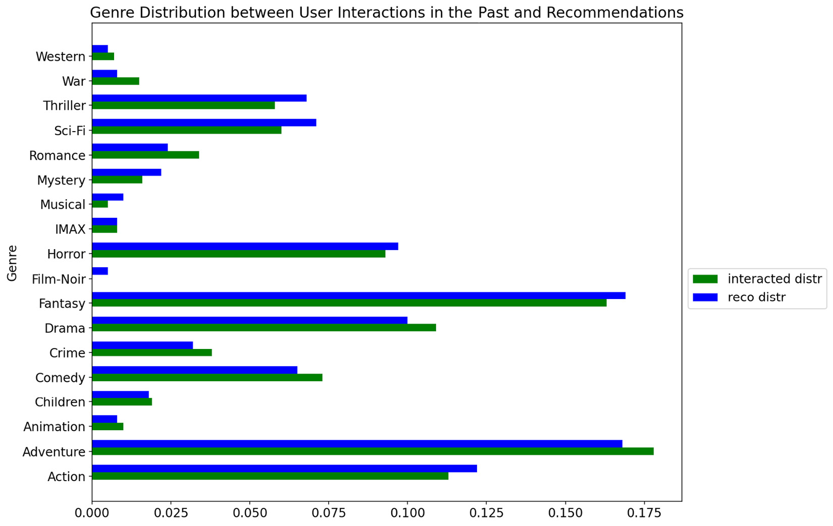
Figure 11.20 – Comparing a user’s historical distribution and calibrated recommendation distribution

In the preceding discussion, we saw the importance of developing a calibrated model due to changes in the input data and the model. Now, let us discuss, from the standpoint of ethical AI, how to incorporate fairness into models and build calibrated models.

Challenges with calibration and fairness

So far, we have learned what it means to have a fair ML model across different population subgroups so that the prediction results are unbiased across all races, ethnicities, genders, and other population categories. From the standpoint of AI ethics, we should also try to design fair and calibrated models, and in the process, try to understand the risks associated with them. To design a fair and calibrated model, it is essential that a group of people assigned a predicted probability of p of generic ML models sees a fair representation. To achieve this, we should have a p fraction of members of this set belonging to positive instances of the classification problem.

Thus, to justify fairness between two groups, G1 and G2 (such as African-American and white defendants), the best way to satisfy both groups is for the calibration condition to hold simultaneously for each individual within each of these groups as well.

However, calibration and error-rate constraints have mutually conflicting goals. Research studies demonstrate that calibration is tolerant only with a single error constraint (which is equal false negative rates across groups). It also becomes increasingly hard to minimize error disparity across different population groups with calibrated probability estimates. Even when the objective is satisfied, the resulting solution resembles a generic classifier, which only optimizes for a percentage of predictions. Thus, to summarize, a perfectly fair and calibrated model cannot be designed.

Summary

In this chapter, we have learned about different ideas related to concept drift. These can be applied to both streaming (batch streams) and live data as well as trained ML models. We also learned how both statistical and contextual methods play an important role in estimating model metrics by determining model drift. The chapter also answered some important questions related to model drift and explainability and helped you to understand model calibration. In the context of calibration, we also learned about fairness and calibration and the limitations of achieving both at the same time.

In the next chapter, we will learn more about model evaluation techniques and handling uncertainties in model-building pipelines.

Ética, Direito e Inteligência Artificial The Ethics of Model Adaptability

Ética, Direito e Inteligência Artificial