In this chapter, we will first set an outline of how fairness has become important in the world of predictive modeling by providing examples of different challenges faced in society. We will then go deep into the taxonomies and types of fairness to present a detailed description of the terms involved. Here, we will understand the importance of the defined metrics by citing and substantiating open source tools that help evaluate the metrics. Then, we will further emphasize the importance of the quality of data as biased datasets can introduce hidden bias in ML models. In this context, this chapter discusses different synthetic data generation techniques that are available and how they can be effective in removing bias from ML models. In addition, the chapter also emphasizes some of the best practices that can not only generate synthetic private data but can also scale and fit different types of problems well.

In this chapter, these topics will be covered in the following sections:

• Understanding the impact of data on fairness
• Fairness definitions
• The role of data audits and quality checks in fairness
• Fair synthetic datasets

This chapter requires you to have Python 3.8 along with some necessary Python packages:

• git clone https://github.com/yoshavit/fairml-farm.git (works with TensorFlow-1.14.0 or TensorFlow-1.15.0
• python setup.py install
• %tensorboard --logdir logs/gradient_tape
• pip install fat-forensics[all] (https://github.com/fat-forensics/fat-forensics)
• pip install fairlens
• git clone https://github.com/amazon-research/minimax-fair.git
• python3 main_driver.py

In this first section, let’s understand what fairness is and how data plays a part in making a dataset fair. By fairness, we mean the absence of any prejudice or favoritism toward an individual or group based on their inherent or acquired characteristics (A Survey on Bias and Fairness in Machine Learning, Ninareh Mehrabi, Fred Morstatter, Nripsuta Saxena, Kristina Lerman, and Aram Galstyan: https://arxiv.org/pdf/1908.09635.pdf). The stated definition emphasizes the presence of certain biases, allowing preferential, unfair treatment toward one individual/sub-group of a population section due to certain attributes, such as gender, age, sex, race, or ethnicity. The goal of the following sections is to avoid creating unfair algorithms that are biased toward a section or group of people.

Real-world bias examples

To study the impact of datasets, let’s see some real-world examples of where and how bias exists and the role of data in creating such biases. One of the most prominent examples where bias is visible is the Correctional Offender Management Profiling for Alternative Sanctions (COMPAS) software. This tool has been used in many jurisdictions around the US to predict whether a convicted criminal is likely to re-offend. The software revealed bias against African-Americans, demonstrating a higher false positive rate for African-American offenders than Caucasian offenders: the former group (African-Americans) exhibits a higher risk of falsely being identified as offenders or repeat criminals than the latter. One obvious reason is the absence of adequate data representations for minority groups. The evidence of racial discrimination has been summarized by ProPublica as follows:

Black defendants were often predicted to be at a higher risk of recidivism than they actually were. Our analysis found that black defendants who did not recidivate over a two-year period were nearly twice as likely to be misclassified as higher risk compared to their white counterparts (45 percent vs. 23 percent).

White defendants were often predicted to be less risky than they were. Our analysis found that white defendants who re-offended within the next two years were mistakenly labeled low risk almost twice as often as black re-offenders (48 percent vs. 28 percent).

The analysis also showed that even when controlling for prior crimes, future recidivism, age, and gender, black defendants were 45 percent more likely to be assigned higher risk scores than white defendants.

Black defendants were also twice as likely as white defendants to be misclassified as being a higher risk of violent recidivism. And white violent recidivists were 63 percent more likely to have been misclassified as a low risk of violent recidivism, compared with black violent recidivists.

The violent recidivism analysis also showed that even when controlling for prior crimes, future recidivism, age, and gender, black defendants were 77 percent more likely to be assigned higher risk scores than white defendants.

(Quoted from How We Analyzed the COMPAS Recidivism Algorithm by Jeff Larson, Surya Mattu, Lauren Kirchner, and Julia Angwin)

The reports published by ProPublica give us a clear idea of the impact of racial discrimination. As the tool is a clear demonstration of injustice against minorities, the dataset present in COMPAS (https://www.kaggle.com/code/danofer/compass-fairml-getting-started/data) is more often used for evaluating fairness in ML algorithms, to check the occurrence of bias, if any.

This kind of bias is more evident in chatbots, employment matching, flight routing, automated legal aid for immigration algorithms, and search and advertising placement algorithms. We can also see such bias is present in AI and robotic systems, face recognition applications, voice recognition, and search engines.

Bias has a detrimental impact on society when the outcomes of biased ML models extend or withhold opportunities, resources, or information (such as hiring, school admissions, and lending). Such issues are most visible in face recognition, document search, and product recommendation, where system accuracy is impacted. End user experiences are impacted when biased algorithmic outcomes generate a feedback loop (due to repeated user interactions with the top items on the list) between data, algorithms, and users, thereby increasing the number of sources yielding further bias.

Note

What is most important for us to know is that when algorithms are trained on biased data, the algorithm itself learns the bias during the training process and reflects that in its predictions.

Now let’s look at Table 7.1 and understand the different sources of bias. Bias resulting from data may come in different forms: data-to-algorithm (DA) bias, algorithm-to-user (AU) bias, and user-to-data (UD) bias.

Table 7.1 – Different types of bias and its sources

Now, with our understanding of different types of bias, let’s see in Figure 7.1 how they are dependent on each other and circulate in a loop. For example, the involvement of user interaction, resulting in behavioral bias, sees its bias amplified when fed with data. The input data adds to aggregation or longitudinal bias. This in turn is processed by algorithms that add bias, termed ranking or emergent bias.

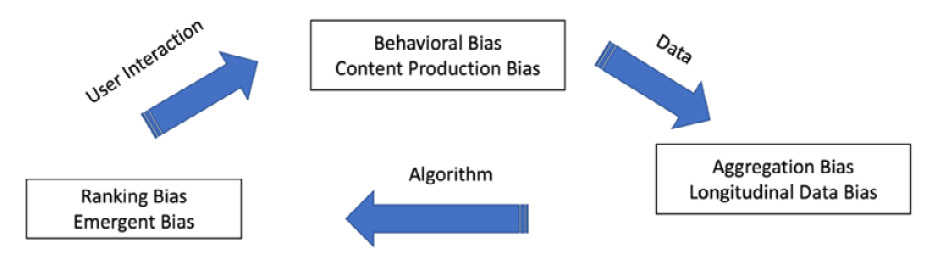
Figure 7.1 – Flow of different types of bias based on sources

Causes of bias

In the following list, we will look at exactly what causes bias:

• Skewed dataset: The dataset may display skewness toward the least-occurring class. This kind of bias tends to increase at a compound rate with time. Crime datasets exhibit this kind of skewness, as we see a very limited number of criminals versus innocent people in any region. Once skewness is observed, detectives and police departments also tend to be biased and dispatch more police professionals to high-crime areas. This may tend to reveal high crime rates, having more police professionals deployed compared to other regions.
• Insufficient training data: We observe that with only limited data for certain demographic groups or other groups, an ML model tends to produce biased outcomes. Such models fail to notice extraordinary characteristics that are available with a very limited population. We saw such examples in Chapter 3, with facial recognition technology having greater accuracy with images of white males compared to images of black females.
• Human bias: Datasets often get corrupted due to human bias. One such example can be seen when we collect real-world data on US employment. Women hardly account for the CEOs in the data on the top 500 companies. This is due to the fact that there are fewer female CEOs and we have failed to collect data where women are CEOs. Models trained on such data would naturally predict that being female correlates poorly with being a CEO.
• Data de-biasing: To remove bias from historical data, we have often seen approaches such as removing sensitive attributes, but that does not completely eliminate bias. Experimental studies reveal correlated attributes are often used as proxies, even after the removal of sensitive attributes that pave the way for the systematic discrimination of minorities. One example of this kind is when a particular locality is predominantly resided in by black people and the removal of the race column does not remove the bias due to the presence of the ZIP code of that location. Possible recommendations to avoid this are to keep the sensitive columns and directly monitor and remediate violations caused by the presence of proxy features during model training.
• Side-effects from data debiasing: Techniques often applied to remove data skewness and model bias sometimes result in undesired side-effects in the model downstream. This has been observed when a speech recognition algorithm was fine-tuned for males and females, with the results significantly worse for female speakers compared to male ones. Researchers further observed that testing models for bias with holdout samples did not solve this, as the test dataset was also biased.
• Availability of limited features: When features are less informative or reliable for minority groups than the counterparts of a majority group, models demonstrate much lower accuracy for the minority section compared to the majority section of the population.
• Diversity among data and AI professionals: It has been found that the absence of diversity has been one of the main causes of bias. Diversity in teams can help to mitigate bias. One study put forward by Joy Buolamwini, founder of the Algorithmic Justice League and past member of MIT Media Lab, demonstrates that certain discoveries were made by her team when a Ghanaian-American computer scientist joined her research group. The team together found out that facial recognition tools exhibited bias and showcased poor performance on her darker skin tone – and only worked if she wore a white mask.
• Costs incurred in driving fairness algorithms: Organizations that have not invested in fairness have more biased ML models. Organizations need to invest in human resource experts and in educating people to opt for fair ML model designs. This may come at the cost of achieving the right trade-off between model accuracy and fairness metrics, which can impact profit margins, revenue, or the number of customers. Hence, it is necessary to balance the two objectives before enforcing regulations.
• External audits: Bias can also arise from the absence of proper external audits. External audits, when put in place, can detect biased datasets or algorithmic bias that’s in place. However, organizing such audits may violate GDPR, CCPA, and other privacy regulations that strictly enforce the privacy of customers’ sensitive data. A workaround is to leverage the use of synthetic data tools that allow you to generate fully anonymous, completely realistic, and representative datasets. An organization can rely on synthetic datasets to train ML models without violating privacy laws, as sharing the data does not disrespect individual privacy.
• Fair models become biased: It often happens in the absence of the constant monitoring of incoming data and model metrics that fair models become biased. One such example is the AI chatbot Tay, developed by Microsoft. Microsoft had to withdraw Tay from the web as it become misogynistic and racist while learning from the conversations of Twitter users. Continuous monitoring and evaluation of model metrics can help to prevent bias from arising over time.
• Biased AI and its vicious cycle: If we fail to measure and assess bias from AI algorithms, it will percolate deep within our society and will potentially be more harmful. One such example was seen with Google’s search algorithm, which displayed racist images on applying searches for terms such as black hands. The searches, instead of perpetuating bias and displaying derogatory depictions, could have showcased more neutral images if the initial search results and the clicks on the search results were not pointed at biased images.

Now, we understand how we can introduce bias while training ML models. We should also be aware of discrimination processes that also yield biased models.

Discrimination is another source of unfairness originating due to human prejudice and stereotyping based on sensitive attributes present in the dataset. Discrimination primarily originates from systems or statistics. Systemic discrimination refers to existing policies, customs, or behaviors within an organization that enhance discrimination against certain subgroups of the population. Statistical discrimination, however, occurs when decision-makers use average group statistics to judge an individual belonging to that group.

Hence, we can say in generating biased ML models that the dataset plays an important role, as it provides the statistics, features, and patterns of data that are learned during the model training phase.

In this section, we studied different types of bias that exist and creep into systems. To avoid bias, we need to incorporate fair treatment for everyone, and in order to do that we need to define what it means to offer fair treatment. Let’s look at that in the next section.

In this section, let’s try to understand the different types of fairness that researchers have described to avoid discrimination or the unfavorable treatment of people. ML algorithms and practitioners are increasingly coming under scrutiny on this subject to mitigate the risk of unfair treatment in areas such as credit, employment, education, and criminal justice. The goal is to design ML algorithms and pipelines that are not impacted by protected attributes (such as gender, race, and ethnicity) but are still able to offer fair predictions. We’ll look at some different fairness definitions with examples.

Numerical and binary attributes are most often used to state and test fairness criteria. Categorical features can be converted to a set of binary features. Most often, we use the terms protected and unprotected groups, advantaged and disadvantaged groups, and majority and minority groups interchangeably to differentiate between the demographic sections of the population and evaluate fairness for different sections of the population. In the definitions discussed in this section, we will primarily use married/divorced female entrants and married/divorced male entrants to demonstrate how preferential treatment or mistreatment can be avoided, to ensure fair and equitable model predictions. Here, entrants mean initial-stage job applicants.

Types of fairness based on statistical metrics

The statistical measures of fairness are dependent on metrics, which can be best explained by means of a confusion matrix – a table that is generated by running predicted outcomes against ground truth data with an actual representation of the different accuracy metrics of a classification model. The rows and columns represent the predicted and the actual classes respectively. For a binary classifier, both predicted and actual classes have two values: positive and negative, as shown in the following figure. The following definitions further illustrate the metrics that are situated in the four different quadrants of the matrix shown in Figure 7.2:

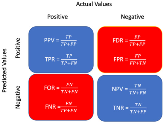
Figure 7.2 – Model classification metrics

True positive (TP)

The model’s predicted outcome and ground truth data are both in the positive class (true, in binary classification).

False positive (FP)

The model’s predicted outcome is true, while the ground truth data is false and belongs to the negative class.

False negative (FN)

The model’s predicted outcome is false and lies in the negative class, while the actual ground truth data is true, belonging to the positive class.

True negative (TN)

The model’s predicted and ground truth data are both false and they lie in the negative class.

Positive predictive value (PPV)/precision

This is the rate of positive cases accurately predicted to be true or lying in the positive class out of all predicted positive cases. It represents the probability of a subject with true as the predicted outcome truly belonging to the same class (having true as the ground truth data), P(Y = 1|d = 1), where an entrant with a good predicted qualifying score actually has a ground truth where the qualifying score is also good.

False discovery rate (FDR)

This is the rate of negative cases that were inaccurately predicted to be true. The FDR represents the probability of false acceptance, P(Y = 0|d = 1), where we observe that a job candidate with a good predicted qualifying score has a ground truth where the person’s qualifying score is actually reported as low.

False omission rate (FOR)

This is the rate of positive cases that were wrongly classified and predicted to belong to the negative class. The FOR represents the probability of samples having a true value being inaccurately rejected, P(Y = 1|d = 0). We observe this most often when a job entrant has been evaluated to have a low predicted qualifying score, but the same candidate in reality has a good score.

Negative predictive value (NPV)

This is the rate of negative samples that are accurately predicted to be in the negative class out of all predicted negative cases. The NPV represents the probability of a subject (or an entrant) with a negative prediction truly belonging to the negative class, P(Y = 0|d = 0).

True positive rate (TPR)

This is the rate of positive samples that are accurately predicted to be in the positive class out of all actual positive cases. The TPR is often referred to as sensitivity or recall; it represents the probability of a truly positive subject being identified in the class it belongs to, P(d = 1|Y = 1). In our example, it is the probability that a job entrant with ground truth data representing a good qualifying score is accurately predicted by the model.

False positive rate (FPR)

This is the rate of negative samples inaccurately predicted by the model to be true, out of all actual negative cases. The FPR represents the probability of false alerts, P(d = 1|Y = 0). An example is when an entrant exhibiting a low qualifying score in reality has been misclassified by the model and inaccurately given a good qualifying score.

False negative rate (FNR)

This is the rate of samples with true values that are mistakenly predicted to be false, out of all actual positive cases. The FNR represents the probability of a negative result given an actual outcome, P(d = 0|Y = 1). An example is when the probability of an entrant having a good qualifying score happens to be wrongly classified.

True negative rate (TNR)

This is the rate of samples with a value of false that are accurately predicted to be in the negative class, out of all actual negative cases. The TNR represents the probability of an outcome being given a false value and actually belonging to the negative class, P(d = 0|Y = 0). We observe this when the probability of an entrant with a low qualifying score happens to be accurately classified.

Let’s calculate these scores on the COMPAS dataset:

1. Let’s first import the necessary Python libraries:

   %matplotlib inline
   from IPython.core.interactiveshell import InteractiveShell
   InteractiveShell.ast_node_interactivity = "all"
   import numpy as np
   import pandas as pd
   import matplotlib.pyplot as plt
   import seaborn as sns
   from sklearn.metrics import confusion_matrix

   CopyExplain
2. Next, we load the data:

   url = 'https://raw.githubusercontent.com/propublica/compas-analysis/master/compas-scores-two-years.csv'
   df = pd.read_csv(url)

   CopyExplain
3. We translate the dataset into a binary classification problem to evaluate whether an individual has a high/medium/low risk of recidivism:

   df['is_med_or_high_risk'] = (df['decile_score']>=5).astype(int)

   CopyExplain
4. Next, we plot the model’s performance after normalizing by each row – we want to see the PPV, FDR, FOR, and NPV:

   cm = pd.crosstab(df[‘is_med_or_high_risk’], df[‘two_year_recid’], rownames=[‘Predicted’], colnames=[‘Actual’], normalize=’index’)
   p = plt.figure(figsize=(5,5));
   p = sns.heatmap(cm, annot=True, fmt=".2f", cbar=False

   CopyExplain

This yields the following output:

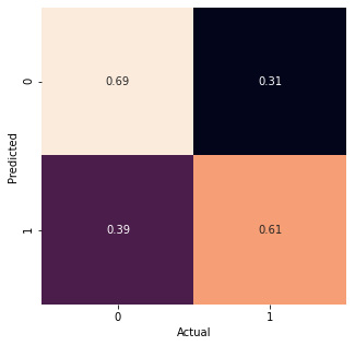
Figure 7.3 – A confusion matrix using the COMPAS dataset

5. We can also print the values using an sklearn confusion matrix:

   [[tn , fp],[fn , tp]]  = confusion_matrix(df['two_year_recid'], df['is_med_or_high_risk'])
   print("True negatives:  ", tn)
   print("False positives: ", fp)
   print("False negatives: ", fn)
   print("True positives:  ", tp)

   CopyExplain
6. Then we concentrate on African-American or Caucasian defendants, since they are the subject of the ProPublica claim:

   df = df[df.race.isin(["African-American","Caucasian"])]
   (df['two_year_recid']==df['is_med_or_high_risk']).astype(int).groupby(df['race']).mean()

   CopyExplain

This yields the following output:

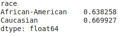
Figure 7.4 – Fairness accuracy metrics for African-American and Caucasian

Here, we see that the fairness metric is not the same across both groups.

Types of fairness based on the metrics of predicted outcomes

The types of fairness listed in this section primarily focus on a predicted outcome for various demographic segments of subjects involved in the problem under consideration.

Group fairness/demographic parity

This is also commonly known as statistical parity or the equal acceptance rate. This concerns whether subjects in both protected (race, gender, ethnicity, and so on) and unprotected groups exhibit an equal probability of being represented in the predicted class classified as true. For example, this condition will be satisfied when there is an equal probability of male and female applicants achieving an equally good predicted qualifying score: P (d =1|G = m) = P (d = 1|G = f).

To illustrate this further, let’s assume an ML model predicts that married/divorced male and female entrants have scores of 0.81 and 0.75, respectively. Here, the classifier can be said to have failed as it fails to satisfy the objective of equal scores for both males and females.

Conditional statistical parity

This definition goes beyond the previous definition by allowing a set of attributes that can influence the model’s predictions. To explain this further, this metric can be satisfied only when both protected and unprotected groups have an equal probability of being designated with the true class. This can be controlled by a set of allowable factors, L (including the entrant’s credit history, employment, and age). Hence, to explain mathematically that both female and male entrants demonstrate an equal probability of achieving a good qualifying score, we state it as follows:

P (d = 1|L = l, G = m) = P (d = 1|L = l, G = f)

However, scores for married/divorced male and female entrants can be found to be very close; for example, they are 0.46 and 0.49, respectively. When we see such a minor difference existing between two groups, we can allow a threshold factor to permit this allowable difference.

Types of fairness based on the metrics of predicted and actual outcomes

The fairness concepts listed here go beyond consideration of what the model predicts as its outcomes, d, for different demographic sections of subjects involved in the process of classification. They go on to compute evaluation metrics that are compared to the actual outcome, Y (as evident in the ground truth data), and recorded in the dataset.

Predictive parity

This concept is very important, and it ensures that a classifier can satisfy that both protected and unprotected groups demonstrate a measure of equal PPV – ensuring that the probability of a subject exhibiting a true or positive predictive value is actually included in the positive class. As an example, we would need to have both male and female entrants demonstrate the same probability score. This can be formulated as:

P (Y = 1|d = 1, G = m) = P (Y = 1|d = 1, G = f)

Furthermore, a classifier with an equal PPV will also have an equal FDR, which means:

P (Y = 0|d = 1, G = m) = P (Y = 0|d = 1, G = f)

The measures may not be fully equal and a threshold margin between the groups is permitted. For example, a classifier may record the PPV for married/divorced male and female entrants as 0.73 and 0.74, respectively, and the FDR for male and female entrants as 0.27 and 0.26, respectively.

In real-world ML algorithms, most often, we find that any trained classifier understands an advantaged group better and predicts them in the positive prediction class. The disadvantaged or minority group’s predicted outcome sees a greater number of challenges in correct evaluation, mostly due to there being limited data for that group.

False positive error rate balance/predictive equality

This metric ensures that the classifier satisfies that both protected and unprotected groups demonstrate similar behavior by exhibiting measures that represent an equal FPR (a metric used for the misclassification rate) – where a subject with a false value and that is included in the negative class possesses a true positive predictive value. For example, this concept implies that both male and female entrants show the same probability measure, which causes entrants with a low qualifying score to be designated a good predicted qualifying score. Mathematically, it can be formulated as:

P (d = 1|Y = 0, G = m) = P (d = 1|Y = 0, G = f)

Here, a classifier with an equal FPR will also exhibit an equal TNR. Hence:

P (d = 0|Y = 0, G = m) = P (d = 0|Y = 0, G = f)

In terms of actual values, the FPR for married/divorced male and female entrants is 0.70 and 0.55, respectively, while the TNR is 0.30 and 0.45, respectively. Any tendency of the classifier to assign good qualifying scores to males who previously had low credit would cause the classifier to break the definitions stated and would result in its failure.

False negative error rate balance/equal opportunity

This concept ensures that a classifier satisfies the condition that both protected and unprotected groups have an equal FNR – where a subject containing a true value and that is included in the positive class actually possesses a negative predictive value. This occurs on account of misclassification. Mathematically, it can be formulated as:

P (d = 0|Y = 1, G = m) = P (d = 0|Y = 1, G = f)

This implies the condition that in both the male and female groups, any entrant possessing a good predicted score has been misclassified and predicted as possessing a low score. A classifier with an equal FNR will also have an equal TPR. Now in terms of equation, the following condition holds, where we see TPR should be same for both males and females:

P (d = 1|Y = 1, G = m) = P (d = 1|Y = 1, G = f)

For example, the FPR and TPR for married/divorced male and female entrants are 0.13 and 0.87, respectively. As the classifier exhibits equal measures of good qualifying scores among males and females, this would lead to equal treatment of the two groups. If the classifier can also satisfy the low scores among the two groups, it will be said to satisfy the condition of group fairness.

Equalized odds/disparate mistreatment

This type of fairness, also commonly known as conditional procedure accuracy equality, enforces a condition of fairness by combining the previous two definitions. It standardizes the error rates for both male and female populations, where a classifier is satisfactory if protected and unprotected groups have an equal TPR and an equal FPR. Hence, this acts as a combination function that ensures equality among both male and female groups, when an entrant with a good qualifying score is also correctly designated a good predicted qualifying score by the model. The probability of an entrant having a low qualifying score in reality has been seen to be inaccurately classified by the model and designated a good predicted qualifying score. Mathematically, it can be formulated as:

P (d = 1|Y = i, G = m) = P (d = 1|Y = i, G = f), i ∈ 0, 1

For example, a classifier exhibiting an FPR for married/divorced male and female entrants as 0.70 can only satisfy disparate mistreatment when it also records a TPR of 0.86 for both males and females. But on the other hand, it shows preferential treatment toward the male group by recording an FPR of 0.80, in contrast to an FPR of 0.70 for the female group. This preferential or biased treatment will cause the classifier to fail to satisfy the condition of equalized odds. Hence, classifiers are often found to satisfy predictive parity but not to satisfy the condition of equalized odds.

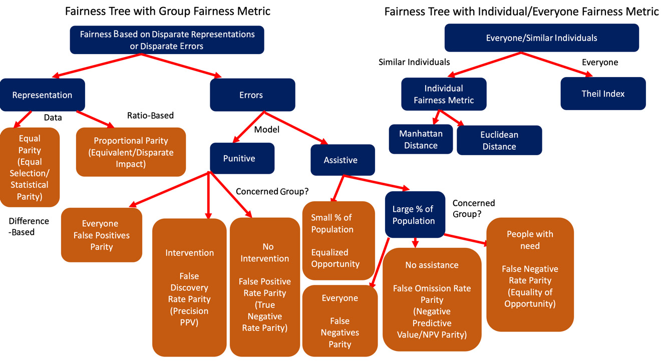
Figure 7.5 – Two fairness trees that represent different types of fairness on group/individual/overall levels

Figure 7.5 gives a condensed representation of these fairness definitions. The preceding figure depicts two fairness trees – the first one is for when we deal with group fairness and the second one is for when we deal with fairness for either individuals or everyone.

The overall fairness metric called the Theil Index is an economic inequality metric used to quantify the divergence of the current distribution of resources (for example, income) within and among diverse demographic groups. Thus, it helps to measure the inequality of income spread (by giving a weighted average of inequality within subgroups) across individuals and groups/sub-groups in a population.

To compute the individual fairness metric, we can either use Manhattan distance (a metric that computes the average Manhattan distance between the samples from two datasets) or Euclidean distance (a metric that computes the average Euclidean distance between the samples from two datasets). For individual fairness, we follow a similar method for similar individuals irrespective of their relationship with any group.

A group fairness tree is generated based on disparate representations or disparate errors. It is based on the two following factors.

Fairness based on disparate representations – equal parity/proportional parity

A fairness tree splits to either equal parity, when we are interested in selecting an equal number of people from each group, or proportional parity, when we are interested in selecting a number of people that is proportional to their percentage in the entire population.

Fairness based on disparate errors in the system – punitive/assistive error metrics

A fairness tree splits to either punitive or assistive error metrics, depending on whether we are interested in making interventions that could either hurt or help individuals.

We further illustrate in Figure 7.6 the computation of group fairness metrics using the Adult dataset (https://archive.ics.uci.edu/ml/datasets/adult).

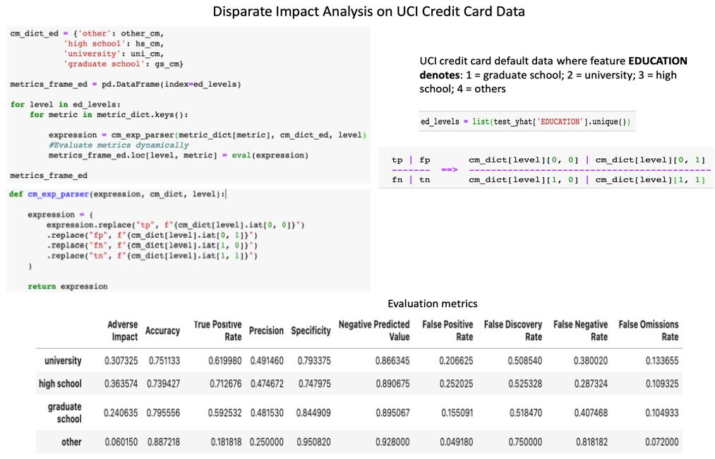
Figure 7.6 – An evaluation of group fairness metrics on the Adult dataset

Conditional-use accuracy equality

This type of fairness is built on the founding principle of joining two equal t” conditions, PPV and NPV. Here, the probability of subjects under consideration having true predictive values in reality is included in the positive class (PPV). We will also observe that the probability of subjects having a false predictive value in reality is included in the negative class (NPV). Mathematically, this can be formulated as:

(P (Y = 1|d = 1, G = m) = P (Y = 1|d = 1, G = f )) ∧ (P (Y = 0|d = 0, G = m) = P(Y = 0|d = 0,G = f ))

Equivalent accuracy is obtained for both male and female entrants. This means that male and female entrants exhibit an equal probability of demonstrating equivalent accuracy values. To explain further, a good predicted qualifying score signals a good qualifying score for an entrant, while a low predicted qualifying score for an entrant signifies a low qualifying score. As with the previous metrics, this one is also not satisfied when the likelihood of a male entrant with a low predicted score diminishes (due to gender bias), causing the male entrant to be given a good qualifying score when he actually should not. A demonstration of this equivalent accuracy metric is that male and female entrants have a PPV of 0.73 and 0.74, respectively, and an NPV of 0.49 and 0.63, respectively.

Overall accuracy equality

This forces a classifier to satisfy the condition that both protected and unprotected groups demonstrate equal prediction accuracy. Here, in the ground truth data, the probability of a subject with values of true or false is classed as either positive or negative. The same class labels are also used in the model’s predictions. This definition implies that true negatives are as desirable as true positives. Mathematically, it can be formulated as:

P (d = Y, G = m) = P (d = Y, G = f)

This metric allows minor differences between males and females, where the two groups exhibit an overall accuracy rate of 0.68 and 0.71, respectively. However, in this example, we consider overall accuracy and not the individual accuracy of predicted classes.

Treatment equality

This metric determines the ratio of errors of the classifier instead of considering its accuracy. As such, the classifier ensures that both the protected and unprotected groups demonstrate an equal ratio of false negatives and false positives (FN/FP), such as 0.56 and 0.62 for male and female entrants, respectively. This idea has been formulated to ensure an equal ratio of false negatives (FN) to false positives (FP) of the different classes of the population for which the ML classifier is being evailuated for fairness.

Types of fairness based on similarity-based measures

Types of fairness built using statistical metrics often suffer from the limitation of ignoring all attributes other than sensitive attributes. This leads to the unfair treatment of one group, even when the same ratio of male and female entrants exhibits the same skillsets or criteria. Such situations arise when selection happens randomly for one group, whereas selection for another group (such as females) is based on certain other attributes (for example, having higher savings). This results in a discrepancy even though statistical parity will mark the classifier as fair. The following types of fairness are put forward to address such issues that may arise due to selection bias by removing the marginalization of insensitive attributes, X, of the classified groups under study.

Causal discrimination

A classifier is said to fulfill the condition of causal discrimination when it produces the same classification for any two subjects with exactly the same features (or attributes), X. To satisfy this criterion, both males and females with identical attributes should either be designated a good qualifying score or a low qualifying score, and this should be the same for both groups. Mathematically, this can be expressed as:

(Xf = Xm ∧ Gf ! = Gm) → df = dm

To test this fairness measure, for each entrant in the test set, we need to generate identical entrants of the opposite gender and compare the predicted classification probabilities for those entrants. The classifier will fail if we fail to achieve the same probabilities for the two groups.

Fairness through unawareness

A classifier is said to fulfill this condition of fairness when no sensitive attributes are explicitly used to predict the final model outcome. Training such models requires that no gender-, race-, or ethnicity-related features are used while training the model. Mathematically, the classification outcome of two similar entrants i and j (of the opposite gender) with identical attributes can be expressed as (X : Xi = Xj → di = dj). To test this condition, for each entrant in the test set, we need to generate identical entrants of the opposite gender and compare the predicted classification probabilities for those two entrants. The classifier is then trained with any classification algorithm (such as logistic regression or a random forest classifier) without using any sensitive attributes and is validated as succeeding if and only if it generates the same probabilities for both groups. However, we also need to ensure that no proxy features of the direct sensitive attributes are used to train the model, which may again result in creating unfair results in the model outcome.

Fairness through awareness

This measure of fairness combines the previous two types to illustrate the fact that similar individuals should exhibit similar classifications. We can evaluate the similarity of individuals based on a distance metric, where the distributions of predicted outcomes for individuals should lie within the computed distance between the individuals. The fairness criterion is said to be satisfied when D(M(x), M(y)) ≤ k (x, y), where V represents the set of entrants, k serves as the distance metric between the two entrants, D (distance) represents the metric between the distribution of predicted outputs, and V × V → R creates an alignment from a set of entrants to probability distributions over outcomes M: V → δA.

Now let’s illustrate this further with an example. As k represents the distance between two entrants i and j, it can hold the value 0 if the features in X (all features/attributes other than gender) are identical, or 1 if some features in X vary. D could be defined as 0 if the classifier resulted in a prediction in the same class, or 1 otherwise. The metric of consideration here is the distance, which has been computed by normalizing the difference between attributes such as age, income, and others. The reduction to a simpler version ensures the easy representation of distance, which is the statistical difference between the model’s predicted probabilities for two entrants: D(i, j) = S(i) − S(j).

Types of fairness based on causal reasoning

The types of fairness that we’ve covered have been designed based on a directed acyclic graph, where nodes represent the attributes of an entrant and edges represent associations between the attributes. Such graphs aid in building fair classifiers and other ML algorithms, as they are driven by the relationships between the attributes and their impact on the model outcomes. The relationships can be further expressed by a different set of equations, to ascertain the impact of sensitive attributes and allow only a tolerance threshold to permit discrimination among different groups present in the population.

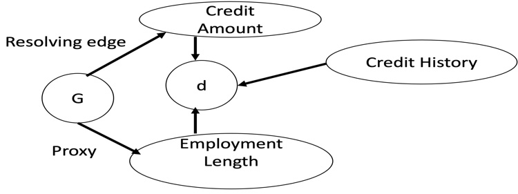
Figure 7.7 – A causal graph with a proxy attribute and a resolving attribute

Figure 7.7 shows a causal graph comprising the attributes credit amount, employment length, credit history, protected attribute G (or gender), and predicted outcome d. Figure 7.7 depicts how a proxy attribute (like G) can be derived from another attribute, which in our case is employment length. As the causal graph demonstrates, we can easily derive the entrant’s gender from their employment duration. Similarly, we use the term resolving attribute in a causal graph to describe an attribute that is determined by a protected attribute, in an unbiased fashion without any discrimination. Credit amount serves as a resolving attribute for G, where the variations observed in credit amount for different values of G are not considered biased and do not hold any discrimination.

Now, let’s look at different types of fairness based on causal reasoning:

• Counterfactual fairness: This type of fairness is applicable to a causal graph when the predicted outcome d in the graph has no dependence on a descendant of the protected attribute G. We see in the example shown in Figure 7.7 that d is dependent on credit history, credit amount, and employment length. Even the presence of a single direct descendant of G, employment length in this case, can cause the model to break the condition of being counterfactually fair.
• No unresolved discrimination: This property exists in a causal graph when there is an absence of any path from the protected attribute G to the predicted outcome d. The presence of a resolving variable can be treated as an exception and is not a violation of anything. In Figure 7.7, there exists a path from G to d via credit amount, which is non-discriminatory. The presence of credit amount enables the establishment of a resolving attribute. It further aids in creating a discriminatory graph by generating a path via employment length. Hence, this graph demonstrates an example of unresolved discrimination and cannot satisfy this type of fairness.
• No proxy discrimination: This property of a causal graph implies that it is devoid of any proxy discrimination. In other words, it means there exist zero paths from the protected attribute G to the predicted outcome d. In the absence of any blockage caused by a proxy variable, the causal graph can be said to have no proxy discrimination, thereby confirming an unbiased representation of the data. However, in our example, there is an indirect path from G to d via the employment length proxy attribute, which means the graph has proxy discrimination.
• Fair inference: This type of fairness in a causal graph helps the path classification process by labeling the paths in a causal graph as legitimate or illegitimate. A causal graph guarantees the satisfaction of the fair inference condition, where illegitimate paths from G to d are absent. However, as Figure 7.7 shows, the existence of another illegitimate path, via credit amount, means it cannot satisfy the condition of fair inference. Employment length is an important factor for consideration in credit-related decisions, so even though it behaves as a proxy candidate for G, the path can be referred to as a legitimate path.

We have studied different statistical measures of fairness, but they alone are insufficient to conclude that the predictions are fair, and they assume the availability of actual, verified outcomes. Despite using statistical metrics, we cannot be certain that outcomes present in training data will always be present in the classified model and that predictions will also conform to the same distribution. More advanced definitions of fairness using distance-based similarity metrics and causal reasoning have also been proposed to support fairness in model predictions, but they require expert intervention to confirm results.

A problem in seeking expert judgments is that they can involve bias. Modern research techniques explore ways to reduce the search space without compromising accuracy. Furthermore, when we try to meet all fairness conditions in a solution, the complexity of the solution increases, as doing so requires the exploration of a larger search space. Fair prediction also requires the consideration of social issues such as unequal access to resources and social conditioning. Teams involved in data processing and ML model development should try to analyze social issues’ impact and incorporate it when designing fair solutions.

With these types of fairness in mind, let’s now try to master some of the open source tools and techniques available to run data audits and quality checks.

Even before digging deep into predictive algorithms and evaluating fairness metrics, we must try to see whether the training data used in the process is skewed and biased toward a majority of the population. This is mainly because most bias results from not having enough data for a disadvantaged or minority sector of a population. Additionally, bias also emerges when we do not apply any of the techniques to deal with data imbalance. In such scenarios, it is essential for us to integrate explainability tools to justify the variability and skewness of the data.

Let’s now investigate how to measure data imbalance and explain variability with the use of certain tools. One of the tools we are going to use first is Fairlens, which aids in fairness assessment and improvement (such as evaluating fairness metrics, mitigation algorithms, plotting, and so on). Some examples are given here with code snippets (on the COMPAS dataset), which will help us to understand the data distributions and evaluate the fairness criteria.

The necessary imports for running all the tests are as follows:

import pandas as pd
import fairlens as fl
df = pd.read_csv""../datasets/compas.cs"")

Assessing fairness

Let’s try out Fairlens:

1. The fairlens.FairnessScorer class can be used to automatically generate a fairness report on a dataset, if you provide it with a target column. Here, the target column stays independent of the sensitive attributes. We can analyze the inherent bias in a dataset used for supervised learning by passing in the name of a desired output column. Now, let’s generate the demographic report of the dataset:

   fscorer = fl.FairnessScorer(df,""RawScor"", ""Ethnicit"",""Se""])
   fscorer.plot_distributions()
   print""Demo Re"", fscorer.demographic_report())

   CopyExplain

This will generate the following output, which shows that there is a complete representation of distributional scores of all the major demographic sections of the population.

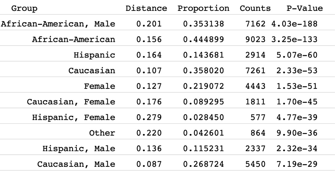
Figure 7.8 – Distribution statistics of the different demographic groups of the population

2. We also plot the distributions of decile scores in subgroups made of African-Americans and Caucasians as shown here:

   group1 = ""rac"": ""African-America""]}
   group2 = ""rac"": ""Caucasia""]}
   fl.plot.distr_plot(df,""decile_scor"", [group1, group2])
   plt.legend(""African-America"",""Caucasia""])
   plt.show()

   CopyExplain

This gives us the following output:

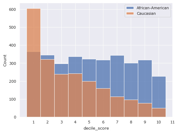
Figure 7.9 – Proportion of two groups – majority and minority

Statistical distance

This is another important distance parameter that we want to consider if we want to evaluate how the distributions between two sensitive demographic groups/sub-groups vary. The metric is used for evaluating the statistical distance between two probability distributions, group1 and group2, with respect to the target attribute.

This can be done using the following code to yield (0.26075238442125354, 0.9817864673203285). It returns the distance and the p-value, as p_value is set to True:

group1 = ""Ethnicity"": ""African-America""]}
group2 = df""Ethnicity""] ==""Caucasia""
print (fl. metrics. stat_distance(df, target_attr, group1, group2, mode""aut"", p_value=True))

Proxy detection

This metric helps us to evaluate proxy features in some datasets. Some insensitive attributes may become highly/partially correlated with sensitive columns, which can effectively become proxies for them. This in turn makes the model biased when the same dataset is used for training. Here, for the four different data points, we can try to evaluate the hidden insensitive proxy features:

col_names = ""gende"",""nationalit"",""rando"",""corr"",""corr""]
data = [
    ""woma"",""spanis"", 715, 10, 20],
    ""ma"",""spanis"", 1008, 20, 20],
    ""ma"",""frenc"", 932, 20, 10],
    ""woma"",""frenc"", 1300, 10, 10],
]
df = pd.DataFrame(data, columns=col_names)
print(fl.sensitive.find_sensitive_correlations(df))

Linear regression

Linear regression can help us to identify proxy features, by evaluating the correlation between the dependent and independent variables.

Cosine similarity/distance method

Cosine similarity is one of the mechanisms used to detect proxy features, where the similarity factor evaluates similar items in multidimensional space. Any two features in a dataset (say, for example, for a loan application dataset) would become proxy features when the cosine similarity between any two vectors falls in the same direction. Such cases seem obvious when we see monthly income and expenditure behaving as proxy features, particularly in a loan application with the applicant’s gender and number of dependents taken together.

The linear association method using variance

This metric was discussed in the paper Hunting for Discriminatory Proxies in Linear Regression Models by Yeom, Datta, and Fredrikson (https://arxiv.org/pdf/1810.07155.pdf) and aims to measure the association between two attributes. To compute this metric, we need to compute cov (X1, X2)2 / Var (X1) Var (X2), which can be done as follows:

1. First, we need to compute the covariance factor between the two feature attributes:

   covar_sex_dur = data.Sex.cov(data.Duration)

   CopyExplain
2. The next step is to compute the individual variances of the feature attributes:

   variance_sex = data.Sex.var()
   variance_dur= data.Duration.var()

   CopyExplain
3. Then we try to evaluate the degree of linear association between the feature attributes:

   association = covar_sex_dur/(variance_sex*variance_dur)
   print ""Association between Sex and Duratio"", association)

   CopyExplain

We get the following output:

Association between Sex and Duration -0.014593816319825929

Now, let’s look at how we determine the correlations between protected features and other features.

The variance inflation factor

The variance inflation factor (VIF) metric aims to measure multicollinearity by evaluating the coefficient of determination (R2) for each variable. As this method determines proxy features, it can aid in removing collinear or multicollinear features, which act as proxies for sensitive/protected attributes in the dataset. Further feature removal can be done by leveraging multiple regression trees.

A high value for VIF in a regression model between protected features and other features would be interpreted as a sign of collinearity between multiple colinear features. Furthermore, it would also indicate the strong presence of another feature that is collinear and thus is a proxy for the feature under study:

1. The first step is to have the necessary library imports for the VIF and load the german_credit dataset:

   import pandas as pd
   from statsmodels.stats.outliers_influence import variance_inflation_factor
   df = pd.read_csv""../datasets/german_credit_data.cs"")
   data = df[''Ag'',''Se'',''Jo'',''Duratio'',''Credit amoun'']]
   data = data.dropna()

   CopyExplain
2. The next step is to create a mapping for the sensitive feature attributes and segregate the independent features for which we want to compute the VIF:

   data''Se''] = data''Se''].map(''mal'': 0,''femal'': 1})
   X = data[''Ag'',''Se'',''Jo'',''Credit amoun'',''Duratio'']]

   CopyExplain
3. The final step is to run the VIF on the data, evaluate the VIF for each feature attribute, and discover the potential proxy features:

   vif_data = pd.DataFrame()
   vif_data""featur""] = X.columns
   vif_data""VI""] = [variance_inflation_factor(X.values, i)
                      for i in range(len(X.columns))]
   print(vif_data)

   CopyExplain
4. We get the following output, which clearly shows that Job and Duration have high VIF values. Using them together leads to a model with high multicollinearity. They serve as potential candidates for proxy features:

              feature    VIF
               Age  5.704637
               Sex  1.365161
               Job  7.180779
      Credit amount 3.970147
           Duration 6.022894

   CopyExplain

Mutual information

This metric signifies the amount of information available for a random feature attribute given another feature attribute is existing. It works in non-linear tree-based algorithms by computing I(X1, X2), which is a weighted sum of joint probabilities, in contrast to COV(X1, X2), which is a weighted sum of the product of the two features:

1. We can compute the mutual information score for the german_credit dataset as follows:

   mi_1 = mutual_info_score(data''Ag''], data''Se''])
   mi_2 = mutual_info_score(data''Jo''], data''Se''])
   mi_3 = mutual_info_score(data''Duratio''], data''Se''])
   mi_4 = mutual_info_score(data''Credit amoun''], data''Se''])
   print""Mutual Inf"", mi_1, mi_2, mi_3, mi_4, mi_5)

   CopyExplain
2. We get the following output, which again confirms the fact that the relationship between credit amount and sex is high, followed by the relationship between the sex and credit duration attributes:

   Mutual Info 0.06543499129250782 0.003960052834578523 0.019041038432321293 0.5717832060773372

   CopyExplain

Significance tests

When we assess fairness scores and evaluate statistical distances, we may also want to test the null hypothesis and see whether the null or alternate hypothesis is true. This can be done using bootstrapping or permutation tests to resample the data multiple times. These iterations compute the statistic multiple times and provide an estimate of its distribution, by computing the p-value or the confidence interval for the metric:

1. Let’s see with the following example how we can compute the confidence interval as well as the p-value between male and female distributions:

   group1 = df[df""Se""] ==""Male"] ""RawScor""]
   group2 = df[df""Se""] ==""Female"] ""RawScor""]

   CopyExplain
2. The test statistic can be configured with the following code. t_distribution can be set up using either the permutation or bootstap method between the two groups previously created:

   test_statistic = lambda x, y: x.mean()–- y.mean()
   t_distribution = fl.metrics.permutation_statistic(group1, group2, test_statistic, n_perm=100)

   CopyExplain

Or, you can use this code:

t_distribution = fl.metrics.bootstrap_statistic(group1, group2, test_statistic, n_samples=100)

3. Now, let’s compute the confidence interval and p-value as shown here:

   t_observed = test_statistic(group1, group2)
   print("Resampling Interval", fl.metrics.resampling_interval(t_observed, t_distribution, cl=0.95))
   print("Resampling Pval", fl.metrics.resampling_p_value(t_observed, t_distribution, alternative="two-sided"))

   CopyExplain
4. Now we get the output that follows. For the first case, we get the confidence interval as a tuple, while for the second case, we receive the p-value:

   Resampling Interval (0.24478083502138195, 0.31558333333333327)
   Resampling Pval 0.37

   CopyExplain

Evaluating group fairness

We have seen how group fairness is important for fulfilling fairness generally. Natalia Martinez, Martin Bertran, and Guillermo Sapiro are the inventors of the concept of the minimax fairness criteria, which aims to improve group fairness metrics. Let’s now study the important concept of minimax fairness (https://github.com/amazon-research/minimax-fair), which strives to achieve fairness when protected group labels are not available. Equality of error rates is one of the most intuitive and well-studied forms of fairness. But using them poses a major challenge when we try to equalize error rates by raising the threshold of error rates, which is undesirable for social welfare causes. Hence, increasing the error margins to establish equal error rates across equally accurate racial groups, income levels, and geographic locations is not a good choice. To further increase group fairness, we can use the minimax group error, proposed by Martinez in 2020. The concept of group fairness does not seek to equalize error rates (as stated earlier in the fairness definitions). Instead, this metric tries to minimize the largest group error rate, to ensure that the worst group demonstrates the same values in terms of fairness metrics. This relaxed concept of fairness tries to achieve the right trade-off between minimax fairness and overall accuracy. The metric has a two-fold objective:

• First, it tries to find a minimax group fair model from a given statistical class
• Then it evaluates a model that minimizes the overall error subject, where the constraint has been set to bind all group errors below a specified (pre-determined) threshold

The objective of the preceding two steps is to reduce the process to unconstrained (non-fair) learning over the same class, where they converge. The minimax fairness metric can be further extended to handle different types of error rates, such as FP and FN rates, as well as overlapping groups having intersectional characteristics. Such groups with intersectional attributes are not just limited to race or gender alone, but can also comprise combinations of race and gender:

1. Using a dataset, we generate X, y, grouplabels, and groupnames:

   X, y, grouplabels, group_names, group_types, is_categorical = 
       setup_matrices(path, label, groups, usable_features=usable_features,
                      drop_group_as_feature=drop_group_as_feature,
                      categorical_columns=categorical_columns, groups_to_drop=groups_to_drop,
                      verbose=verbose,
                      save_data=save_data, file_dir=file_dir, file_name=file_name)

   CopyExplain
2. Here X and y are the features and labels for each type of group. Furthermore, X is divided into a number of different groups, where each of which has a shared linear function. This function is used to sample the labels with noise. In the absence of a dataset, to build and evaluate a fair minimax of a model, we can employ a synthetic data generation mechanism, as in the following code snippet:

   generate_synthetic_data(numdims, noise, numsamples=1000, num_group_types=1, min_subgroups=2, max_subgroups=10, min_subgroup_size=20, mean_range=0, variability=1, num_uniform_features=0, intercept_scale=2, binary=False, drop_group_as_feature=False, save_data=False, file_dir='', file_name='', random_seed=0)

   CopyExplain
3. Now the learning process can be kicked off as in the following code snippet, with the parameters necessary for learning given in the table that follows:

   minimax_err, max_err, initial_pop_err, agg_grouperrs, agg_poperrs, _, pop_err_type, total_steps, _, _, _, 
   _, _, _ = 
       do_learning(X, y, numsteps, grouplabels, a, b, equal_error=False,
                   scale_eta_by_label_range=scale_eta_by_label_range, model_type=model_type,
                   gamma=0.0, relaxed=False, random_split_seed=random_split_seed,
                   group_names=group_names, group_types=group_types, data_name=data_name,
                   verbose=verbose, use_input_commands=use_input_commands,
                   error_type=error_type, extra_error_types=extra_error_types, pop_error_type=pop_error_type,
                   convergence_threshold=convergence_threshold,
                   show_legend=show_legend, save_models=False,
                   display_plots=display_intermediate_plots,
                   test_size=test_size, fit_intercept=fit_intercept, logistic_solver=logistic_solver,
                   max_logi_iters=max_logi_iters, tol=tol, penalty=penalty, C=C,
                   n_epochs=n_epochs, lr=lr, momentum=momentum, weight_decay=weight_decay,
                   hidden_sizes=hidden_sizes,
                   save_plots=save_intermediate_plots, dirname=dirname)

   CopyExplain

Let’s now see the different parameters and their functionalities involved in fair synthetic data generation:

Table 7.2 – Different parameters for training the minimax model

Figure 7.10 shows the variation of individual group errors, group weights, and the average population error with synthetic data using minimax group fairness with logistic regression. We can see that both the individual sub-groups (log-loss errors) and average population error (log loss) roughly follow the same trend and remain confined between 0.63 and 0.65.

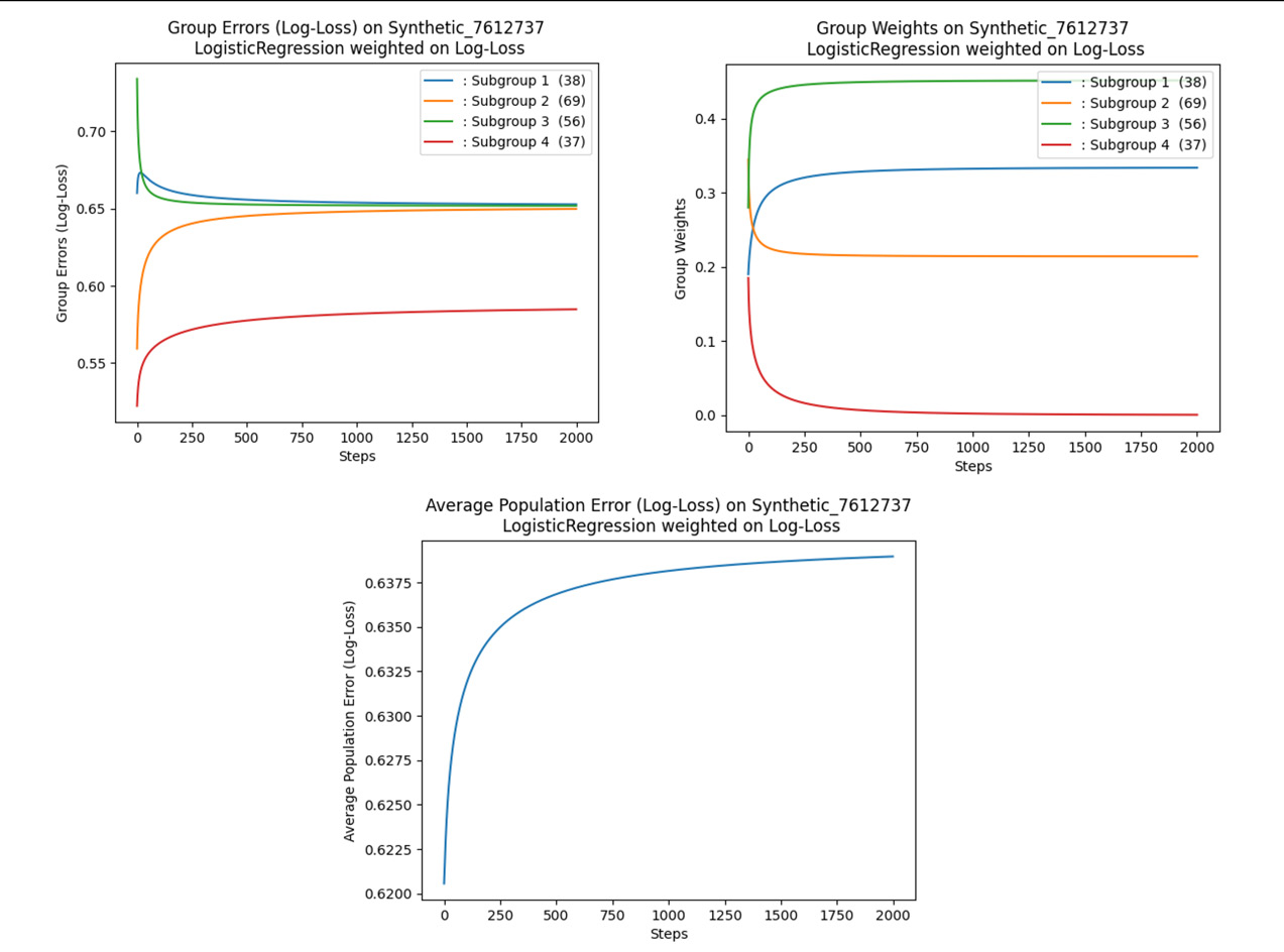
Figure 7.10 – A diagram showing different parameters for training the minimax model

Evaluating counterfactual fairness

Let’s use the open source FAT Forensics (fatf) library, which is a Python toolbox that can be used for evaluating the fairness, accountability, and transparency of predictive systems:

1. Let’s first set up the necessary imports:

   import numpy as np
   import fatf.utils.data.datasets as fatf_datasets
   import fatf.utils.models as fatf_models
   import fatf.fairness.predictions.measures as fatf_pfm
   import fatf.transparency.predictions.counterfactuals as fatf_cf

   CopyExplain
2. Let’s load a synthetic healthcare dataset:

   hr_data_dict = fatf_datasets.load_health_records()
   hr_X = hr_data_dict['data']
   hr_y = hr_data_dict['target']
   hr_feature_names = hr_data_dict['feature_names']
   hr_class_names = hr_data_dict['target_names']

   CopyExplain
3. With the dataset loaded, let’s map the target indices to target names, dropping unnecessary columns, before starting the training process:

   hr_y = np.array([hr_class_names[i] for i in hr_y])
   unique_identifiers = ['name', 'email', 'zipcode', 'dob']
   columns_to_keep = [i for i in hr_X.dtype.names if i not in unique_identifiers]
   hr_X = hr_X[columns_to_keep]
   hr_feature_names = [i for i in hr_feature_names if i not in unique_identifiers]

   CopyExplain
4. Next, we start the model training and select instances for counterfactual fairness:

   clf = fatf_models.KNN()
   clf.fit(hr_X, hr_y)

   CopyExplain
5. After training the model, let’s select the data instances (its protected features) for which we would like to test the counterfactual fairness:

   data_point_index = 4 + 2
   data_point = hr_X[data_point_index]
   data_point_y = hr_y[data_point_index]
   protected_features = ['gender', 'age']

   CopyExplain
6. Print out the protected features and instances:

   assert protected_features, 'The protected features list cannot be empty.'
   person = ' is' if len(protected_features) == 1 else 's are'
   print('The following fautre{} considered protected:'.format(person))
   for feature_name in protected_features:
       print('     "{}".'.format(feature_name))
   print('nEvaluating counterfactual fairness of a data point (index {}) of '
         'class *{}* with the following features:'.format(data_point_index,
   data_point_y))
   for feature_name in data_point.dtype.names:
       print('     The feature *{}* has value: {}.'.format(
           feature_name, data_point[feature_name]))

   CopyExplain

This results in the following output:

The following features are considered protected:
     "gender".
     "age".
Evaluating counterfactual fairness of a data point (index 6) of class *fail* with the following features:
     The feature *age* has value: 41.
     The feature *weight* has value: 73.
     The feature *gender* has value: female.
     The feature *diagnosis* has value: heart.

7. The next step is to compute the counterfactually unfair samples:

   cfs, cfs_distances, cfs_classes = fatf_pfm.counterfactual_fairness(
       instance=data_point,
       protected_feature_indices=protected_features,
       model=clf,
       default_numerical_step_size=1,
       dataset=hr_X)

   CopyExplain
8. The final step is to print the counterfactually unfair data points:

   cfs_text = fatf_cf.textualise_counterfactuals(
       data_point,
       cfs,
       instance_class=data_point_y,
       counterfactuals_distances=cfs_distances,
       counterfactuals_predictions=cfs_classes)
   print('n{}'.format(cfs_text))

   CopyExplain
9. This generates the following output:

   Counterfactual instance (of class *success*):
   Distance: 19
       feature *age*: *41* -> *22*
   Counterfactual instance (of class *success*):
   Distance: 20
       feature *age*: *41* -> *22*
       feature *gender*: *female* -> *male*

   CopyExplain

We have already studied what disparate impact is when looking at fairness. Now let’s see with code examples how we can measure the three most common disparate impact measures.

10. To evaluate the equal accuracy metric, we can use the following code snippet:

    equal_accuracy_matrix = fatf_mfm.equal_accuracy(confusion_matrix_per_bin)
    print_fairness('Equal Accuracy', equal_accuracy_matrix)

    CopyExplain
11. To evaluate the equal opportunity metric, we run the following:

    equal_opportunity_matrix = fatf_mfm.equal_opportunity(confusion_matrix_per_bin)
    print_fairness('Equal Opportunity', equal_opportunity_matrix)

    CopyExplain
12. To evaluate the demographic parity metric, we run this:

    demographic_parity_matrix = fatf_mfm.demographic_parity(
        confusion_matrix_per_bin)
    print_fairness('Demographic Parity', demographic_parity_matrix)

    CopyExplain
13. Here is the output we receive on running an evaluation of equal accuracy, equal opportunity, and demographic parity:

    The *Equal Accuracy* group-based fairness metric for *gender* feature split is:
         The fairness metric is satisfied for "('female',)" and "('male',)" sub-populations.
    The *Equal Opportunity* group-based fairness metric for *gender* feature split are:
         The fairness metric is satisfied for "('female',)" and "('male',)" sub-populations.
    The *Demographic Parity* group-based fairness metric for *gender* feature split is:
         The fairness metric is >not< satisfied for "('female',)" and "('male',)" sub-populations.

    CopyExplain

As we have learned about the basics of fairness with examples, we should also find out how to apply these concepts to follow best practices.

Best practices

We have explored with different examples and code snippets the process by which we can evaluate different fairness metrics. However, before evaluation, we need to ensure that the data used for training our models proportionally represents all different demographic groups of the population. Furthermore, to address the issue of fairness, another important criterion is to ensure that your predictions are calibrated for each group (https://towardsdatascience.com/understanding-bias-and-fairness-in-ai-systems-6f7fbfe267f3). When model scores are not calibrated for each group, we may end up overestimating or underestimating the probability of outcomes for different groups. We may need to redesign thresholds and create separate models and decision boundaries for each group. This process will alleviate bias and enable fairer predictions for each of the groups than a single threshold.

Most of the time, we are not able to get data where all groups of the population are equally represented. In such situations, the best practice is to generate synthetic datasets by applying artificial methods, so that we not only train the model with equal representations of the different groups but are also able to validate the predicted outcomes against different thresholds customized for each group. This will eliminate representation bias and account for geographic diversity while creating such datasets.

We also have certain tools, mentioned next, for evaluating fairness.

Bias mitigation toolkits

Here is a list of some tools:

• Aequitas: An open source bias and fairness audit toolkit that evaluates models for different types of bias and fairness metrics on multiple population sub-groups.
• Microsoft Fairlearn: This toolkit takes the reduction approach to fair classification (e.g. binary classification) by leveraging constraints. The constraint-based approach reduces fair classification problems to a sequence of cost-sensitive classification problems. Under applied constraints, this yields a randomized classifier, with the lowest (empirical) error.
• The What-If Tool: This open source TensorBoard web application is a toolkit provided by Google that allows you to view the counterfactuals to analyze an ML model. Users are then able to compare a given data point to the nearest data point that resembles it, yet for which the model predicts a different result. This tool also comes with the flexibility of adjusting the effects of different classification thresholds, along with the ability to tweak different numerical fairness criteria.
• AI Fairness 360: This toolkit, developed by IBM, contains an exhaustive set of fairness metrics for datasets and ML models. It comes with explainability for these metrics, and different algorithms to mitigate bias in datasets at the preprocessing and model training stages.

We discuss some of these toolkits in later chapters.

Now that we know about the different bias mitigation toolkits that are available, and how important auditing data and running frequent quality checks is, let’s study synthetic datasets and how they can help in modeling fair ML problems.

By synthetic data, we mean data generated artificially from scratch, with statistical properties matching the original or base dataset that is ingested into the system. A synthetically generated dataset bears no relationship to the real subjects present in the original dataset.

Modern research in artificial intelligence (AI) has led to innovations and the publication of advanced tools that can generate synthetic data in data-intensive environments. With the availability of better tools and techniques, fair, privacy-preserving synthetic data generation (with tabular data) has been widely adopted by organizations.

Synthetic data-generating algorithms are capable of ingesting real-time data and learning its features, different feature correlations, and patterns. They can then generate large quantities of artificial data that closely resembles the original data in terms of statistical properties and distributions. By and large, these newly generated datasets are also scalable, privacy-compliant, and can display all valuable insights, without violating data confidentiality rules. AI-generated synthetic data is widely used by financial and healthcare providers for scaling their AI solutions. Synthetic data has also been successful in generating robust replacements for missing and hard-to-acquire data.

Sensitive data has often been kept confined to teams and departments. But with the implementation of synthetic-data-generation tools, it has become easier to establish collaboration with teams and third parties in a privacy-compliant manner using private synthetic copies of data. Synthetic data is great for improving ML algorithms that are impacted by bias or imbalances due to new, rare incoming data, which has a greater influence than historic data. This type of synthetic data finds application in determining fraudulent transactions, whose volume is < 5% of the overall transactions. Up-sampled synthetic datasets are not only capable of detecting bias in transactional data but can also comply with ethics and help ML models to yield better, fairer results for minority or disadvantaged groups. Hence, synthetic data serves as a very important component in the design of ethical ML pipelines. Fair synthetic data can remove societal and historical bias from the predictions of ML models.

Now, let’s study, with an example, a framework that generates private synthetic data by using realistic training samples, without disclosing the PII of individuals.

MOSTLY AI’s self-supervised fair synthetic data generator

This framework takes into consideration fairness constraints, in a self-supervised learning process, to simulate and generate large quantities of fair synthetic data. The framework is made following a generative model architecture that feeds in a dataset (in our example, the UCI Adult Census dataset) to get a better dataset that has a higher degree of fairness than the original dataset.

Furthermore, the resultant dataset preserves all the original relationships between the attributes but only controls the gender and racial biases present in the original data. The propensity scores of the predicted model outcomes demonstrate the fact of how fair synthetic data can alleviate bias when compared with the original dataset.

In ML, we often use generative deep neural networks that use new, synthetic samples (that are representations of the actual data) to optimize the accuracy loss of an ML model being trained. The loss can represent the similarity of the fitted function to the observed distributions of the real data. The process of generating fair, representative data involves an additional loss to the original loss function that can penalize any violation of the statistical parity.

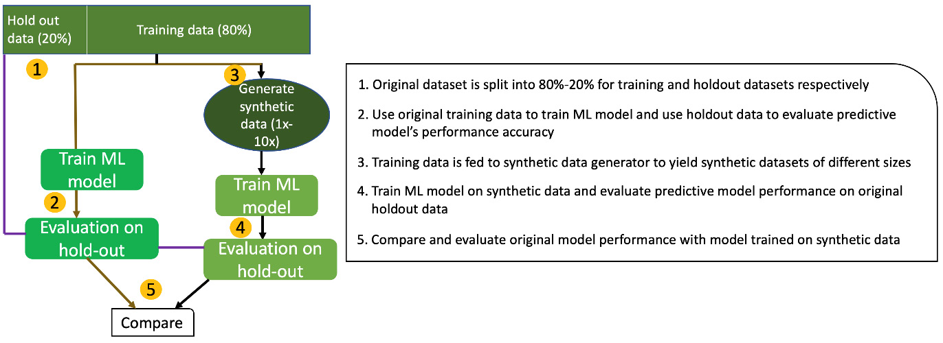
Figure 7.11 – Different parameters for training the minimax model

Hence, the algorithm for fair synthetic data generation involves optimizing a combined loss, which contains the following:

• A weighted sum of the accuracy loss
• A fairness loss that is proportional to the deviation from the empirically estimated statistical parity
• The right trade-off between accuracy and fairness, where weights are shifted from one loss component to the other

Figure 7.11 illustrates the step-by-step sequences of generating synthetic data and comparing model performance when models are trained on original datasets versus synthetic datasets.

We have seen how ML-based synthetic data generation is possible. Now, let’s see how protected attributes such as gender and income in fair synthetic data help to satisfy some of the fairness definitions we studied before.

Influence on fairness statistics

We will leverage a generative deep neural network as a data synthesizer for tabular data to generate synthetic data samples from the adult_income dataset. The generative model synthesizer runs end to end 50 times with a parity fairness constraint and takes gender as a protected attribute. Figure 7.12 shows that the gender imbalance present in the original data within the high-income class is successfully mitigated by the synthetic data. The disparate impact (derived by comparing the difference and the high-income-male-to-high-income-female ratio) is observed to be roughly 10/30 = 0.33 in the original dataset, while it is recorded as 22/25 =0.88 in the bias-corrected synthetic dataset. We see that this metric with synthetic data is considerably higher than 0.80, which is the industry benchmark. We can safely conclude that data synthesis helps in mitigating bias.

We further observe that the additional parity constraint during model training did not reduce the data quality, as shown in Figure 7.12.

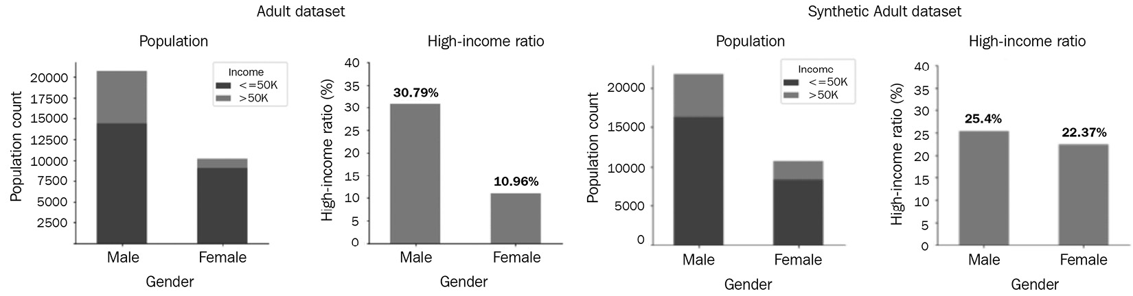
Figure 7.12 – Synthetic data mitigating the income gap

Both the univariate and bivariate distributions demonstrate that the dataset is able to preserve both the population-wide male-to-female and high-earner-to-low-earner ratios. Only the statistical parity constraint signifying the dependence of income and sex has been allowed to be violated to make them un-correlated. With representative and synthetic data, this correlation is reduced to the noise level evident in the following figure (see the red circle on the light green figure).

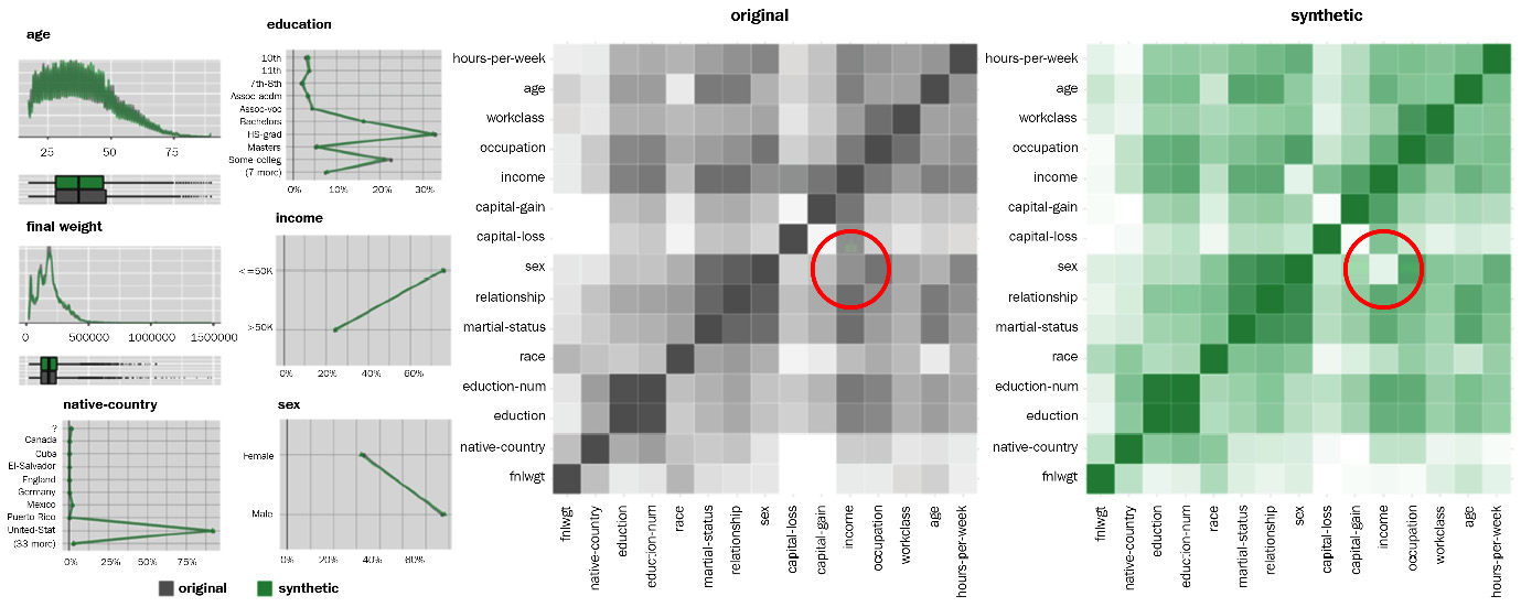
Figure 7.13 – Univariate versus bivariate statistics for original and synthetic data

Studying proxy attributes further shows that they do not introduce unfairness through a backdoor. Even the addition of a strongly correlated artificial feature (correlated with gender) named “proxy” is found to exhibit a constant correlation with “sex” in the original dataset, which is considerably reduced with the introduction of parity constraints due to induced fairness. The female section shows that “proxy” equals 1 in 90% of cases and equals 0 for the remaining 10%. Figure 7.14 further illustrates this:

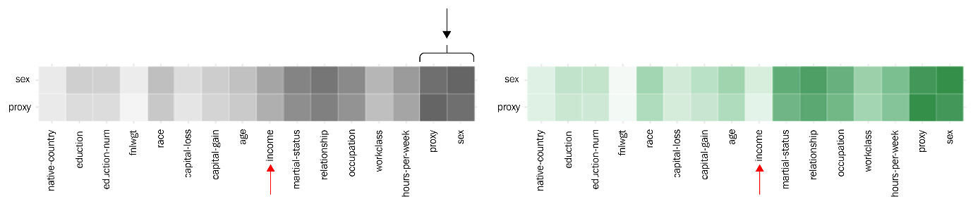
Figure 7.14 – The parity fairness constraint holds good for proxy attributes such as gender

For the Adult dataset, the generative model is trained by applying fairness constraints on “gender” and “race.” Furthermore, it is evident from Figure 7.15 that the synthetic data exhibits highly balanced high-income ratios across all four groups by race and gender. Even though the solution is not able to guarantee complete parity, it can be obtained (when the difference further diminishes) by assigning a higher weight to the fairness loss in comparison to the accuracy loss.

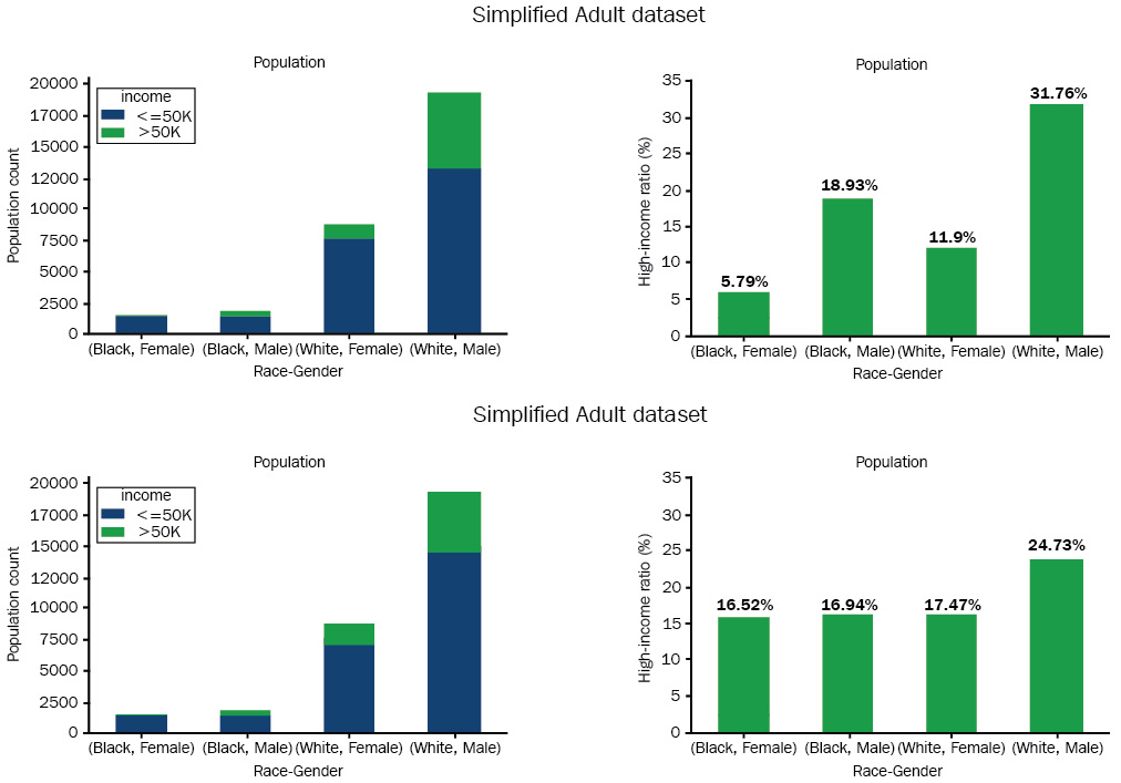
Figure 7.15 – Constraint-based bias mitigation by accounting for gender and race, respectively

In Figure 7.16, we see the propensity scores of the corresponding predictive models, on both the original dataset and the synthetic dataset.

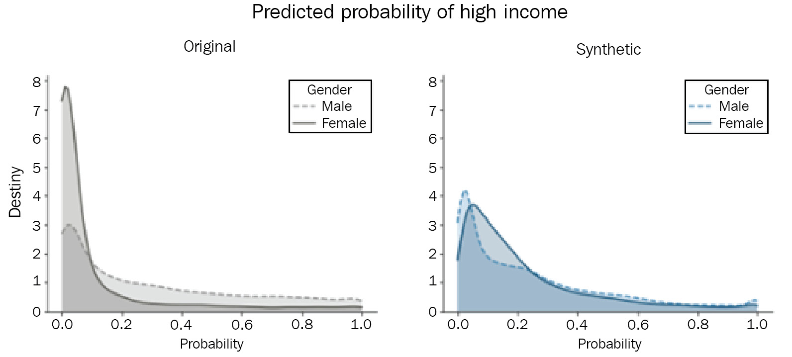
Figure 7.16 – Prediction of high income for both the original and synthetic datasets

Using the same ML model, we find that the model fitted on the original dataset exhibits a much lower probability score for women being in the high-income class when compared with the opposite gender – men. Hence, the discrepancy with synthetic data is reduced and both distributions driven by the gender attribute are found to align. As the training process of the predictive model does not include any model optimization through fairness, it is obvious that the predicted outcome is largely due to using bias-corrected synthetic data. A fairness-constrained synthetic data solution ensures group fairness. The dataset maintains the relationship between other attributes and at the same time removes dependencies between sensitive and target attributes. Furthermore, the parity constraint also ensures fairness for hidden proxy attributes.

The following steps illustrate step by step how to generate fair synthetic data to equally represent males and females:

1. We will set up a specified set of hyperparameters (including input training data size, layer sizes, and classifier types) that we will train using synthetic data:

   inputsize = train_dataset["data"]. shape[1]
   layersizes = [100]
   classifier_type = "paritynn"
   hparams = {
       "classifier_type": classifier_type,
       "layersizes": layersizes,
       "inputsize": inputsize,
   }

   CopyExplain
2. Our next task is to set up a classifier that will train the network using the hyperparameters used in the previous state. While training the dataset, we use the validation dataset to validate the training process:

   classifier = construct_classifier(hparams, loaddir=loaddir)
   classifier.train(train_dataset, logdir, epochs=args.epochs,]
   validation_dataset=validation_dataset)
   savepath = classifier.save_model(logdir)
   n = validation_dataset["label"].shape[0]

   CopyExplain
3. The construct_classifier function is set inside the fariml-farm library to construct the classifier, as given in the following code snippet:

   classifier_types = [SimpleNN, ParityNN, AdversariallyCensoredNN]
   def construct_classifier(hparams, sess=None, loaddir=None):
       for c_type in classifier_types:
           if c_type.name == hparams["classifier_type"]:
               classifier = c_type(sess=sess)
               classifier.build(hparams=hparams)
               if loaddir is not None:
                   classifier.load_model(loaddir)
               return classifier

   CopyExplain
4. Our next job is to enable an equivalent representation of male (1) and female (0) points through the synthetic data generation process:

   n_males = sum(validation_dataset["label"])
   limiting_gender = n_males > n - n_males
   n_limiting_gender = sum(validation_dataset["label"] == limiting_gender)
   max_points_per_gender = 500
   n_per_gender = min(max_points_per_gender, n_limiting_gender)
   inds = np.concatenate([
       np.where(validation_dataset["label"] == limiting_gender)[0][:n_per_gender],
       np.where(validation_dataset["label"] != limiting_gender)[0][:n_per_gender]],
       axis=0)
   vis_dataset = {k:v[inds, ...] for k, v in validation_dataset.items()}
   val_embeddings = classifier.compute_embedding(vis_dataset["data"]

   CopyExplain
5. The classifier is optimized using a loss function, given by the following:

   overall_loss = crossentropy +
           self.hparams["dpe_scalar"]*dpe +
           self.hparams["fnpe_scalar"]*fnpe +
           self.hparams["fppe_scalar"]*fppe +
           self.hparams["cpe_scalar"]*cpe +
           self.hparams["l2_weight_penalty"]*l2_penalty

   CopyExplain

The overall loss is the sum of losses, computed by demographic parity discrimination (dpe), false negative parity (fnpe), false positive parity (fppe), and calibration parity loss (cpe). The loss function evaluated for dpe represents the loss due to demographic_parity_discrimination, while fnpe and fppe represent the loss due to equalized_odds_discrimination.

6. Now if we try to plot the embeddings, we can use the following code snippet, which generates an almost equivalent representation of embeddings between male and female with an annual income >= 50K or < 50K:

   plot_embeddings(val_embeddings,
                   vis_dataset["label"],
                   vis_dataset["protected"],
                   plot3d=True,
                   subsample=False,
                   label_names=["income<=50k", "income>50k"],protected_names=["female", "male"])

   CopyExplain

This produces the following output:

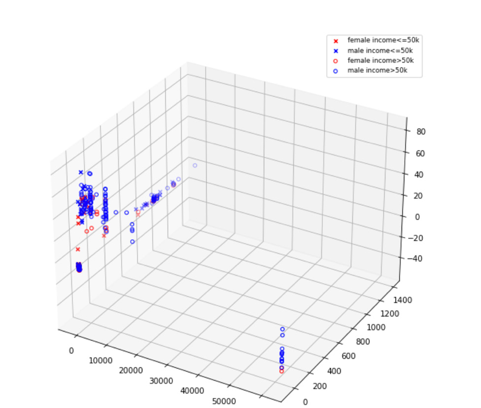
Figure 7.17 – An equivalent representation of embeddings between the male and female populations with an annual income >= 50K or < 50K

We learned how MOSTLY AI’s fairness GANs are capable of generating synthetic datasets that have a positive impact on fairness statistics. Let’s explore a GAN-based approach that uses a directed acyclic graph (DAG) to generate fair synthetic data.

A GAN-based fair synthetic data generator

Now let’s see with an example how we can use causally aware generative networks to generate fair, unbiased synthetic data. The objective is to generate an unbiased dataset with no loss of the representation of the data distribution. The data-generation process can be further modeled by a DAG. Here, the ML model (a single model or a cascade of models) being trained on synthetic data not only gives unbiased predictions (satisfying the fairness criteria) on synthetic data but is also capable of yielding unbiased predictions on real-life available datasets.

The Debiasing Causal Fairness (DECAF) framework, based on GAN, explores the principle of causal structure for data synthesis by employing d generators (each generator being assigned to each variable) to learn about the causal conditionals present in the data. The data-generation process (DGP) embedded within DECAF allows variables to be re-engineered and regenerated based on their origin, which is the causal parents, through the input layers of the generator. A framework like this can remove bias from biased real-world datasets (datasets that under-represent minority groups) with inherent bias and real-world datasets where bias has been synthetically introduced. Furthermore, DECAF promises to offer protection for confidential information through private synthetic data generation processes by swapping out the standard discriminator for a differentially private discriminator.

The discriminator and generator run the optimization process in successive iterations by adding a regularization loss to both networks. The optimization process uses gradient descent and guarantees the same convergence criteria as standard GANs. The framework involves the following:

• A data-generating distribution function that satisfies Markov compatibility. For a known DAG (G), if we find that each node represents a variable in a probability distribution (P), it is said to be Markov-compatible if each variable X present in the DAG is independent of all its non-descendants.
• Enough capacity for both the generator G and discriminator D.
• Every training iteration successfully optimizes a given DAG G and correspondingly updates it.
• Maximized discriminator loss.
• A distribution function generated by the generator that gets optimized to converge it on the true data distribution.

During the training stage, DECAF learns about the causal conditionals that are present in the data with a GAN. The GAN is equipped to learn about causal conditions in the DAG between the source and destination nodes. At the generation (inference) stage, the framework functions by applying three fundamental principles, CF debiasing, FTU debiasing, and DP debiasing, which help the generator to create fair data. However, it is also assumed that the DGP’s graph G is known from before.

During inference, the variable synthesis process originates from the root nodes, then propagates down to their children (from the generated causal parents in the causal graph). The topological process of data synthesis is dependent on the sequential data generation technique, which terminates at the leaf nodes. This enables the DECAF algorithm to remove bias strategically at inference time by enforcing targeted/biased edge removal and further increases the probability of meeting the user-defined fairness requirements. DECAF is also found to satisfy the fairness/discrimination definitions we discussed earlier and at the same time maintains the high utility of generated data so that it can be effectively used by ML models without creating algorithmic bias.

Fairness through unawareness (FTU) is measured by keeping all other features constant and computing the distinctions between the predictions of a downstream classifier, when the classifier’s predictions are either 1 and 0, respectively, such that | PA = 0 (Yˆ|X)–– PA = 1(Yˆ|X) |. This metric helps to evaluate the direct impact of A on the predicted outcomes. This metric aims to eliminate disparate treatment, which is legally related to direct discrimination, and strives to provide the same opportunity to any two equally qualified people, independent of their race, gender, or other protected attributes.

Demographic parity (DP) is measured in terms of the total variation, which signifies and explains the differences between the predictions of a downstream classifier. This helps to compute the positive-to-negative ratio between varying categories (African, American, Asian, and Hispanic, for instance) of a protected variable A:

| P (Yˆ |A = 0)–− P (Yˆ |A = 1) |

This metric does not allow any indirect discrimination unless otherwise provided by explainability factors.

Conditional fairness (CF) aims to generalize both FTU and DP.

All DECAF methods yield good data quality metrics: precision, recall, and AUROC. One good fair data generation mechanism that deserves special mention is DECAF-DP, which performs best across all five of the evaluation metrics (precision, recall, AUROC, DP, and FTU) and has better DP performance results, even when the dataset exhibits high bias.

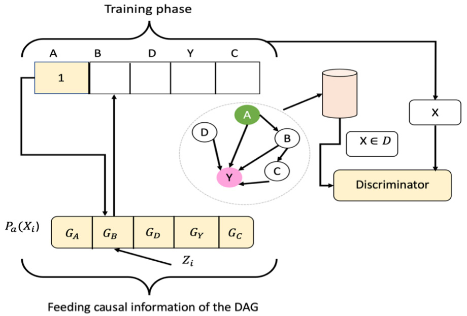
Figure 7.18 – Training phase in DECAF

The training phase from the preceding figure directly follows the inference phase in the following diagram.

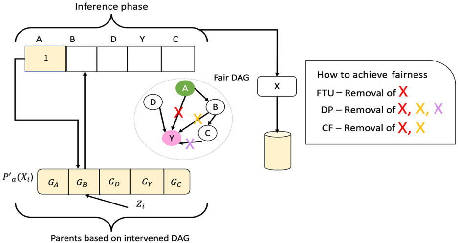
Figure 7.19 – Fairness inference phase enabling fair data synthesis in DECAF

Now let’s see how we can generate synthetic data with DECAF using the following code snippets:

1. The following code is for all necessary imports:

   import networkx as nx
   import pytorch_lightning as pl
   from utils import gen_data_nonlinear
   import sys
   from decaf import DECAF
   from decaf.data import DataModule

   CopyExplain
2. Now, after setting up the necessary imports, let’s set up the DAG structure using dag_seed. The causal structure of the graph is stored in dag_seed:

   dag_seed = [[1, 2], [1, 3], [1, 4], [2, 5], [2, 0], [3, 0], [3, 6], [3, 7], [6, 9], [0, 8], [0, 9], ]

   CopyExplain
3. The next step is to have DiGraph invoked with dag_seed, using the following code snippet. The dag structure is stored in the dag_seed variable. The edge removal is stored in the bias_dict variable. Here, we have removed the edge between 3 and 6. Furthermore, gen_data_nonlinear is used to apply a perturbation at each node:

   bias_dict = {6: [3]}
   G = nx.DiGraph(dag_seed)
   data = gen_data_nonlinear(G, SIZE=2000)
   dm = DataModule(data.values)
   data_tensor = dm.dataset.x

   CopyExplain
4. In the next stage, we set up the different hyperparameters required to facilitate the training process:

   x_dim = dm.dims[0]
   z_dim = x_dim
   lambda_privacy = 0
   lambda_gp = 10
   l1_g = 0

   CopyExplain
5. The weight decay is initialized, which is used by AdamW, an optimizer that is an improved version of Adam (Adaptive Moment Estimation) and is capable of yielding better models with a faster training speed using stochastic gradient descent. AdamW has a weight decay functionality that can be used to regularize all network weights:

   weight_decay = 1e-2

   CopyExplain
6. The next step is to set up the proportion of points to generate, which is negative for sequential sampling:

   p_gen = (-1)
   use_mask = True
   grad_dag_loss = False
   number_of_gpus = 0

   CopyExplain

WGAN-GP

You can read more about the Wasserstein GAN with gradient penalty (WGAN-GP) here: https://jonathan-hui.medium.com/gan-wasserstein-gan-wgan-gp-6a1a2aa1b490.

7. Now let’s initialize and train the DECAF model by setting the different hyperparameters, the generator, and the regularization parameters:

   model = DECAF(
       dm.dims[0],
       dag_seed=dag_seed,
       h_dim=args.h_dim,
       lr=args.lr,
       batch_size=args.batch_size,
       lambda_privacy=lambda_privacy,
       lambda_gp=lambda_gp,
       d_updates=args.d_updates,
       alpha=args.alpha,
       rho=args.rho,
       weight_decay=weight_decay,
       grad_dag_loss=grad_dag_loss,
       l1_g=l1_g,
       l1_W=args.l1_W,
       p_gen=p_gen,
       use_mask=use_mask,
   )
   trainer = pl.Trainer(
       gpus=number_of_gpus,
       max_epochs=args.epochs,
       progress_bar_refresh_rate=1,
       profiler=False,
       callbacks=[],
   )
   trainer.fit(model, dm)
   synth_data = (
       model.gen_synthetic(
           data_tensor, gen_order=model.get_gen_order(), biased_edges=bias_dict
       ).detach()
       .numpy()
   )

   CopyExplain

We have now generated synthetic unbiased data that can be fed to any ML model.

In this chapter, we have learned about the importance of fairness algorithms in resolving societal bias, as different types of bias hinder the ability of an ML model to yield a fair outcome. We had a deep dive to learn about all the different types of fairness and how they can be practically applied to perform data quality checks, discover conditional dependencies and attribute relationships, and generate audit reports. In the process, we looked at how bias may appear in the data itself and/or in the outcome of predictive models. Furthermore, we took the first step in learning about fair synthetic data generation processes that can help in removing bias.

In later chapters, we will learn more about the mechanisms of applying fairness-aware models on diverse datasets, or diverse groups within a population. In addition, we will also look at the proper selection of protected attributes (such as gender, race, and others) based on the domain space of the problem and the dataset under study. In our next chapter, Chapter 8, Fairness in Model Training and Optimization, we will learn more about creating constrained optimization functions that can help in building fair ML models.

• Fairness Definitions Explained in Proceedings of the International Workshop on Software Fairness (FairWare ‘18), Association for Computing Machinery, Verma Sahil and Julia Rubin (2018), https://fairware.cs.umass.edu/papers/Verma.pdf
• A survey on datasets for fairnessaware-machine learning. Wiley Interdisciplinary Reviews: Data Mining and Knowledge Discovery. 10.1002/widm.1452, https://www.researchgate.net/publication/355061634_A_survey_on_datasets_for_fairness-aware_machine_learning
• Representative & Fair Synthetic Data, Tiwald, Paul & Ebert, Alexandra & Soukup, Daniel. (2021), https://arxiv.org/pdf/2104.03007.pdf
• Minimax Group Fairness: Algorithms and Experiments. Proceedings of the 2021 AAAI/ACM Conference on AI, Ethics, and Society. Association for Computing Machinery, New York. Emily Diana, Wesley Gill, Michael Kearns, Krishnaram Kenthapadi, and Aaron Roth. 2021. https://assets.amazon.science/9d/a9/e085008e45b2b32b213786ac0149/minimax-group-fairness-algorithms-and-experiments.pdf
• A Survey on Bias and Fairness in Machine Learning. ACM Comput. Surv. 54, 6, Article 115 (July 2022), Mehrabi Ninareh, Fred Morstatter, Nripsuta Saxena, Kristina Lerman, and Aram Galstyan. (2021). https://arxiv.org/pdf/1908.09635.pdf
• FAT Forensics: A Python Toolbox for Algorithmic Fairness, Accountability and Transparency, Sokol, K., Santos-Rodríguez, R., & Flach, P.A. (2019). https://arxiv.org/pdf/1909.05167.pdf
• Minimax Pareto Fairness: A Multi Objective Perspective, Martinez Natalia, Martin Bertran, Guillermo Sapiro, http://proceedings.mlr.press/v119/martinez20a/martinez20a.pdf