This chapter starts with the introduction of the AI/ML workflow. The chapter then delves into different ML algorithms used for classification, regression, generation, and reinforcement learning. The chapter also discusses issues related to the reliability and trustworthiness of these algorithms. We start with an introduction to the various components of an ML pipeline and explain the need for continuous training. The chapter then briefly explores the important AI/ML algorithms for the tasks of classification, regression, and clustering. Further, we discuss approaches for identifying bias in learning algorithms and causes of uncertainty in model prediction.

In this chapter, these topics will be covered in the following sections:

• Understanding different components of ML pipelines
• ML tasks and algorithms
• Causes of uncertainty in model prediction
• Uncertainty in classification algorithms
• Uncertainty in regression algorithms

Further, we will write Python code to quantify both aleatoric and epistemic uncertainty for regression tasks.

This chapter requires you to have Python 3.8, along with some necessary Python packages:

• TensorFlow 2.7.0
• NumPy
• matplotlib
• Keras-Uncertainty – to install it, use the following:

  !pip install --user git+https://github.com/mvaldenegro/keras-uncertainty.git

  CopyExplain

As any data scientist knows, ML is only as good as the data it’s trained on. In the real world, data is messy and complicated. Building a successful ML system, therefore, requires more than just building algorithms. It also requires a vast and complex infrastructure to support it. This includes everything from collecting and cleansing data to deploying and monitoring models. The problem is further complicated by the fact that changing anything in the system can have ripple effects throughout. A minor tweak in hyperparameters, for example, can require changes to the way data is collected and processed. As a result, building a successful ML system is an immensely complex undertaking.

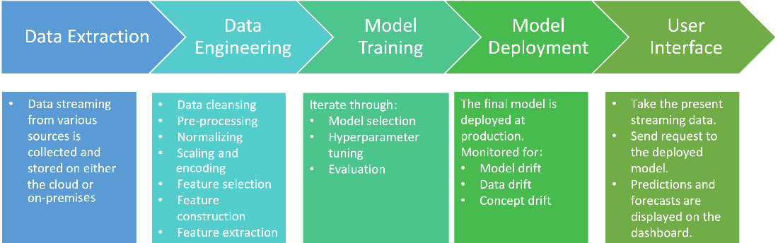
Figure 5.1 – ML workflow

We can divide the ML workflow into five main components:

• Data Extraction: This is the phase where data needed for training the model is curated. It is the process of identifying relevant information from a larger dataset and converting it into a format that can be used for further analysis. This can be done manually, but it is more commonly done using automated algorithms. Data extraction can be used to extract contact information from a list of emails, to identify trends in stock prices, or to find new potential customers. The data can be in different forms (tabular data, image files, text, and so on). The data is decided on by the business needs of the specific use case. For example, if your use case is AI for retail, you will have data such as product pictures and tags. The process of data extraction typically begins with pre-processing, which involves identifying the relevant information from the dataset. Once the relevant information has been identified, it is then converted into a format that can be used by the ML algorithm. It allows the algorithm to focus on the most relevant information and ignore irrelevant data. This can improve the accuracy of the ML algorithm and help to speed up the training process.
• Data Engineering: In this phase, the data is analyzed, cleaned, explored, and pre-processed to be fed to the model. The phase may involve combining one or more features and/or dimensionality reduction of the data for computational efficiency. The goal of data engineering is to create a dataset that is both accurate and representative of the real world in a reproducible way.
• Model Training: This is an iterative phase, where model experiments are performed. It involves selecting the best model, performing hyperparameter tuning, and validating the trained model using desired metrics. Finding the right set of hyperparameters is an art and, in earlier days of ML, only some experts were able to do it effectively. As a result, many used to call ML “alchemy.” However, today, with the availability of robust and reliable optimizers and AutoML features, we can generate reliable and reproducible results. It is worth mentioning, though, that this step is time- and compute-intensive.
• Model Deployment: The final model is deployed to production. It is important to monitor the model’s performance and for any degradation in the performance to be reported and acted upon. The deployed model needs to be monitored for both data drift and concept drift. We will talk about these concepts in detail in Chapter 6.
• User Interface: Once the model is deployed, it is ready for consumption. It will take user input and perform predictions, which can be shared via the visual dashboards.

Depending upon the level of expertise and need, different components of the ML pipeline can be done manually, automated as MLOps (for details, refer to Chapter 6), or fully automated as CI/CD processes.

In general, ML tasks can be categorized into four categories: classification, regression, clustering, and dimensionality reduction (Figure 5.2).

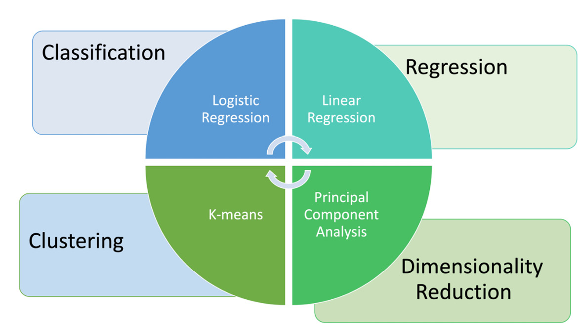
Figure 5.2 – Different ML tasks and popular algorithms

For each of them, there exist many standard algorithms. For the sake of completeness, we will list ML tasks and some common algorithms for them:

• Classification: When data needs to be divided into different categories or classes, we use classification algorithms. This is a supervised learning problem where the aim is to predict the discrete class label of new examples, based on training data. It is one of the most commonly used techniques in ML, and has a wide range of applications, from identifying spam emails to facial recognition. The basic idea behind classification is to build a model that can learn the relationship between the input data and the class labels. This model can then be used to make predictions on new data points. There are a variety of different algorithms that can be used for classification, each with its own strengths and weaknesses. The choice of algorithm will largely depend on the nature of the data and the required accuracy of the predictions.
• Regression: In ML, regression is a technique used to predict continuous values, such as prices or weights. It assumes that there is a linear relationship between the predictor variables and the response variable. In other words, as the predictor variables increase, the response variable will also increase (or decrease) by a constant amount. Regression models can be used to identify which predictors are most important for determining the value of the response variable. They can also be used to estimate uncertainty in the predictions. Despite its simplicity, regression is a powerful tool that can be used to solve many real-world problems. Regression, like classification, is a supervised learning problem.
• Clustering: Clustering is a ML technique that groups similar data points together. It is used to segment customers, classify documents, and identify patterns in data. There are a variety of clustering algorithms, but they all operate on the same principle: they partition data into groups, called clusters, by finding similarities between data points. Clustering is an unsupervised learning technique, which means that it does not require labeled data. This makes it particularly well-suited for exploratory data analysis. Clustering can be used to find structure in data, generate hypotheses about how the data is organized, and identify outliers. By grouping together similar data points, clustering can simplify complex datasets and make them easier to work with. Clustering is an essential tool for ML and data science. It can be used alone or in combination with other techniques to solve a variety of problems. Many clustering algorithms, such as k-means, are based on an unsupervised learning paradigm.
• Dimensionality Reduction: In ML, dimensionality reduction is the process of reducing the number of features in a dataset. This can be done for a variety of reasons, such as reducing the training time or improving the model’s performance. There are a number of different methods for dimensionality reduction, and the most appropriate method will depend on the dataset and the desired results. Some common methods include Principal Component Analysis (PCA) and Linear Discriminant Analysis (LDA). In general, dimensionality reduction can be a useful tool for improving ML models. However, it is important to carefully select the right method for the specific dataset and desired results. Otherwise, it can harm the model’s performance.

The following table lists some of the commonly used algorithms and deep learning models used for each task.

Table 5.1 – A table of ML algorithms

The algorithms listed in Table 5.1 use either supervised learning or unsupervised learning paradigms. However, there is a third paradigm of ML, Reinforcement Learning (RL). It has been explored to train artificial agents to play games, for self-driving cars, and in AutoML to find the best models and hyperparameters for different tasks.

Additionally, in recent years, researchers have developed AI algorithms that can be used to generate data (for example, generative adversarial networks, variational autoencoders, diffusion models, and so on). These algorithms have been explored to generate text, images, art, and much more.

Each of these algorithms has its strengths and weaknesses, so choosing the optimal algorithm for a task often requires you to iterate through different algorithms and choose the one giving the best performance in terms of the evaluation metrics. However, to build a responsible AI solution, it is important that models are also evaluated against bias and fairness, and that the end user is made aware of the uncertainty in the predictions of the model.

In the next section, we will talk about uncertainty and how to estimate uncertainty in model prediction.

ML is inseparably connected with uncertainty. After all, machines learn from data that is itself uncertain. This data might be noisy, incomplete, or just plain wrong. As a result, any conclusions that the machine draws from this data are going to be subject to some degree of uncertainty. And thus, we need to be aware of the inherent uncertainty in any results that we obtain and account for it appropriately. Only then can we hope to make the best use of ML in our decision-making processes. To make this point, here is a prediction using EfficientNet, one of the top-scoring networks on the ImageNet dataset (Tan and Le, 2019).

EfficientNet receives the following image:

Figure 5.3 – Input to EfficientNetB0 from the ImageNet dataset

It returns the following output:

Predicted: [('n04326547', 'stone_wall', 0.81027746)]

As you can see, on being presented with a photo of wooden logs, the model predicts it as 'stone_wall' with 81% confidence.

Before we delve further into uncertainty in ML, it would be nice to remember how we humans deal with uncertainty. If you are asked a question – let’s say “What is the NASDAQ index today?” – if you have been following the stock market, you will give either its value or probably say it is bullish or bearish, as the case may be. But if you are not into the stock market, you will simply say “I don’t know.” ML algorithms, however, will give a prediction irrespective of the input. So, if you have an ML algorithm trained to classify flowers, it will tell you what flower you are, even though human identification is not its domain. It would be wonderful if our ML models could also say “Sorry, I do not know – it is not in my domain!” Consider, for example, the self-driving car: it should be able to tell the driver “Hey, I am not sure if what I am seeing is a pedestrian or not. Can you take control?” This becomes even more crucial when we are using deep learning models for crucial decision making, such as providing a loan, providing medical facilities, and so on.

One way to deal with this problem is to quantify uncertainty in the prediction so that when making a prediction a model will tell us how confident it is about its prediction or how reliable its predictions are. In this section, we will explore some of the ways the uncertainty of a model can be quantitatively described. But first, let us see what the different types of uncertainty are and what causes them.

Types of uncertainty

In ML, we often talk about two different types of uncertainty. The first type is aleatoric uncertainty, which refers to the inherent noise in data. This might be, for example, the fact that two people who are measuring the same thing will get slightly different results. Another type of uncertainty is epistemic uncertainty, which refers to our lack of knowledge about the model itself. For instance, if we’re trying to predict the price of a stock, there will always be some uncertainty due to the fact that we can’t know everything about the stock market. Uncertainty is an important part of ML, and understanding the different types can help us build better models.

Let’s delve deep into the types of uncertainty.

Aleatoric uncertainty

Aleatoric uncertainty represents the uncertainty that exists because of the random nature of natural processes. It is inherent uncertainty, present due to probabilistic variability. For example, when tossing a coin, there will always be a certain degree of uncertainty in predicting whether the next toss will be heads or tails. We can never eliminate this uncertainty, no matter how much data we have. To give another example, if we’re trying to predict the weather, there will always be some uncertainty due to the chaotic nature of the atmosphere. There is no way to remove this uncertainty. In essence, every time you repeat the experiment, the results will have certain variations.

Epistemic uncertainty

Epistemic uncertainty comes from the lack of knowledge or a lack of information. There can be various reasons for a lack of knowledge, for example, inadequate understanding of underlying processes, incomplete knowledge of the phenomena, and so on. This type of uncertainty can be reduced.

For example, you can get more data, conduct more experiments, and so on. You can also try to reduce the uncertainty by using a more powerful model or training the model for longer.

Predictive uncertainty

In ML, we are mostly concerned with the uncertainty that is propagated in a prediction, also called predictive uncertainty. On the basis of input data, predictive uncertainty is of three types:

• In-domain uncertainty: The cause of this uncertainty is unequal training data distribution, for example, having more samples of class A as compared to class B. This uncertainty can be reduced by improving the data quality.
• Domain-shift uncertainty: This uncertainty arises when the training data distribution varies significantly from the real-world situation. For example, a model trained to recognize faces does not work well when the faces are occluded, the person is wearing glasses, a cap, or a face mask, and so on. It is possible to improve the model by including data-occluded samples in training.
• Out-of-domain (OOD) uncertainty: As the name suggests, this is uncertainty that arises when the input is drawn from a completely unknown subspace. For example, if we train a model on dog photos and present it with a human, our ML algorithm is unable to tell that the input is outside of the domain it has learned.

Causes of uncertainty

There can be various causes of uncertainty (for more details, you should refer to the publication by Zio and Pedroni, 2012 – see the Further reading section):

• Lack of knowledge: In a supervised learning task, this can be translated as a lack of data that can encapsulate the relationship between input and output. This can be quantitative – for example, we may not know the probability distribution of features – or qualitative, where the features and their distribution are known but the features to describe the problem are unknown. By gaining more data, working closely with experts in the domain can reduce this cause of uncertainty.
• An abundance of data: While today there is no dearth of data that one can save and access, the problem is finding features that are relevant to the use case. Rigorous feature engineering and data exploration can help in selecting relevant features.
• The conflicting nature of data: When we build a ML model, the input features and the output variables are supposed to have some form of a cause-and-effect relationship. However, despite expert knowledge, we can never be sure that the correlations we are seeing in the data are also causation. An interesting example of funny correlations can be found on this site: https://www.fastcompany.com/3030529/hilarious-graphs-prove-that-correlation-isnt-causation.
• Measurement errors: The measurement of physical quantities via sensors always has some level of uncertainty due to the nature of the measuring device itself.
• Linguistic ambiguity: It is often the case that words have different meanings in different contexts. Despite great advancements in natural language processing and new transformer architecture (Vaswani, 2017) that can converse almost like a human being (https://blog.google/technology/ai/lamda/), we still do not have systems that can understand the complexities of human language.
• The subjectivity of analyst opinions: Finally, there is the human factor. There can be uncertainty due to the subjective interpretation of the data analyst. The same piece of data may result in different interpretations depending on the cultural background and competence of the data analyst.

As we can see, while there are ways to reduce some of the causes of uncertainty, it is not possible to completely eliminate them. Therefore, in the rest of this part of the chapter, we will find ways to quantify and ways to reduce uncertainty in different ML tasks.

Quantifying uncertainty

We can divide the deep neural network uncertainty quantification methods available in the literature into four types. They are based on the number (single or multiple) and the nature (deterministic or stochastic) of the deep neural networks used. Figure 5.4 shows the different types of uncertainty quantification methods in the literature.

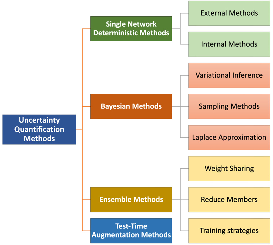
Figure 5.4 – Different uncertainty quantification methods

Let us understand each of these methods:

• Single-Network Deterministic Methods: Conventional neural networks have their weights fixed after training and therefore, for the same input, each prediction results in the same result. In single-network deterministic methods, one works with conventional neural networks, but to add the uncertainty score to the model, one can modify the network by changing the architecture or loss function (internal methods). Alternatively, there are approaches (external methods) where the model and training are not changed. Instead, uncertainty is measured using additional components, for example, training two neural networks, one for the actual prediction task and a second one for the prediction of uncertainty in the first network’s prediction.
• Bayesian Methods: These methods make use of the Bayesian approach. In variational inference methods, the general approach is to approximate the posterior distribution by optimizing over a family of tractable distributions. This is done by minimizing the KL divergence. The sampling methods are based on Markov chain Monte Carlo approaches. Laplace approximation methods work by approximating the log-posterior distribution and, based on it, deriving a normal distribution over the weight of the network.
• Ensemble Methods: These make use of more than one conventional deterministic neural network. Predictions from several models are combined into one prediction. Since the method depends on a variety of ensembles, the variety can be introduced by using random initialization and data shuffling. Using methods such as bagging and boosting to vary the distribution of training data and data augmentation are some of the common ways to have multiple models.
• Test-Time Augmentation Methods: Here, the idea is to create multiple test data from the original test data using the technique of data augmentation. Augmented test data allows the exploration of different views and enables the capturing of uncertainty.

Out of the four, single-network deterministic methods are very straightforward, easy to implement, and computationally less expensive. A lot of interest in recent years has been generated in Bayesian methods, and with the availability of frameworks such as TensorFlow Probability, it has become easier to experiment with them.

Let us consider a sensor whose output can be modeled by a linear process, defined by the relationship y = x.

Let us say we sample data for x lying in the range [-2.5,2.5]. Now, there would always be some noise introduced because of the inherent physical processes of the sensor (for example, white noise). Additionally, the sensor may have limitations such as temperature or pressure requirements. The following graph shows data from our sensor:

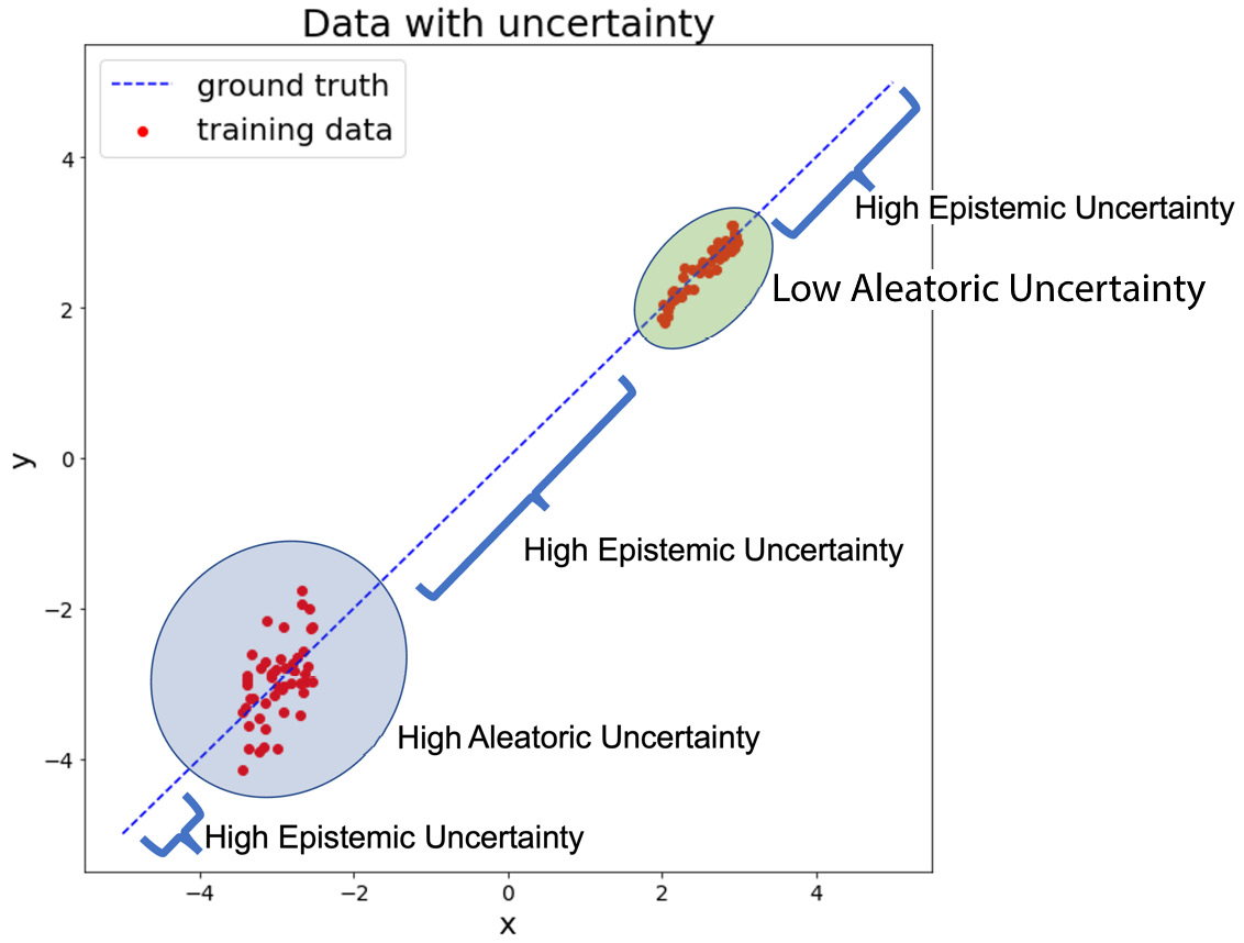
Figure 5.5 – Different kinds of uncertainty in data

We can see that in the lower-left corner, due to some malfunction, there is high aleatoric uncertainty. Also, there are large gaps where there is no observed training data, which can cause high epistemic uncertainty in that range of inputs.

Before we talk about measuring these uncertainties, let us build a model and train it on the training data.

We use TensorFlow Dense layers to build the model. We start with an input layer and then add the hidden layers using the for loop, along with the Dropout layer after each hidden layer, finally followed by a Dense output layer:

def build_model(layers_shape, input_dim, output_dim):
    inputs = Input(shape=(input_dim,))
    hidden = Dense(layers_shape[0], activation='relu', kernel_regularizer=l2(0.004))(inputs)
    hidden = Dropout(0.05)(hidden, training=True)
    for i in range(len(layers_shape)-1):
        hidden = Dense(layers_shape[i+1], activation='relu', kernel_regularizer=l2(0.004))(hidden)
        hidden = Dropout(0.05)(hidden, training=True)
    outputs = Dense(output_dim)(hidden)
    model = Model(inputs, outputs)
    return model
model = build_model(layers_shape=[5,10,20,10,5], input_dim= 1, output_dim=1)
model.summary()

An important point to note here is that the Dropout layers have the training parameter set to the True value. What this means is that dropout will be applied even during inference, and as a result, we will get a variation in predictions. The model summary is as follows:

Model: "model"
______________________________________________________
 Layer (type)             Output Shape         Param #
======================================================
 input_1 (InputLayer)    [(None, 1)]              0
 dense (Dense)            (None, 5)               10
 dropout (Dropout)        (None, 5)               0
 dense_1 (Dense)          (None, 10)             60
 dropout_1 (Dropout)      (None, 10)             0
 dense_2 (Dense)          (None, 20)             220
 dropout_2 (Dropout)      (None, 20)             0
 dense_3 (Dense)          (None, 10)             210
 dropout_3 (Dropout)      (None, 10)             0
 dense_4 (Dense)          (None, 5)              55
 dropout_4 (Dropout)      (None, 5)              0
 dense_5 (Dense)          (None, 1)              6
======================================================
Total params: 561
Trainable params: 561
Non-trainable params: 0
______________________________________________________

We use the rmsprop optimizer, and use the mean square error as the loss function:

model.compile(optimizer='rmsprop', loss='mse', metrics=['mae'])

And we train it using the training data plotted (red dots) in Figure 5.5:

history = model.fit(x_data, y_data, batch_size=10, epochs=200, shuffle=True, verbose=1)

The following graph (Figure 5.6) shows the evolution of loss as the training progresses. We can see that the model learned quite early, and after roughly 25 epochs there is no significant decrease in the loss function:

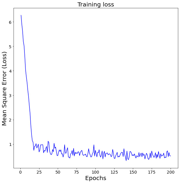
Figure 5.6 – Training loss as the model learn

Let us now see how this model performs on test data. We take input as varying in the range [-10, 10]:

x_test = np.linspace(-10,10,100)
y_pred = model.predict(x_test)

Let us plot the data:

fig, ax = plt.subplots(1,1,figsize=(10,10))
ax.scatter(x_data, y_data, s=10, label='train data', color='red')
ax.plot(x_test, x_test, ls='--', label='ground truth', color='blue')
ax.plot(x_test, y_pred, label='Model Prediction - R2 {:.2f}'.format(r2_score(x_test, y_pred)), color='green')
ax.set_xlabel('x')
ax.set_ylabel('y')
ax.legend()
ax.set_title('Model performance on test data');

The following plot shows the performance on the test dataset:

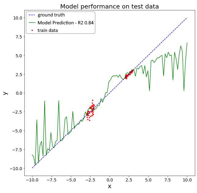
Figure 5.7 – Model performance on test dataset

We can see that on the test data, the R2 score is 0.98. For the most part, this is a great model. However, as we said earlier, there are regions of high epistemic and high aleatory uncertainty in the data.

Let us first explore epistemic uncertainty. We evaluate our model on the test dataset about 500 times, meaning that we predict 500 times using our trained model on the same test data. This is equivalent to simulating a Gaussian process. Each time, we obtain a range of output values for each input scalar from test data. As a result, we can calculate the standard deviation of the posterior distribution and display it as a measure of epistemic uncertainty:

predictions = []
for _ in range(500):
  predictions += [model.predict(x_test,verbose=0)]
mean, std = np.mean(np.array(predictions), axis=0), np.std(np.array(predictions), axis=0)
fig, ax = plt.subplots(1,1,figsize=(10,10))
ax.plot(x_test, x_test, ls='--', color='green', label='test data')
ax.scatter(x_data, y_data, color='blue', label='train data')
ax.set_title('{} - R2 {:.2f}'.format('Epistemic Uncertainity', r2_score(x_test, mean)))
ax.set_xlabel('x')
ax.set_ylabel('y')
ax.fill_between(np.squeeze(x_test), np.squeeze(mean+1*std), np.squeeze(mean-1*std),  alpha=0.4, label='Epistemic Uncertainty', color='orange')
ax.legend();

Figure 5.8 shows the epistemic uncertainty for our model:

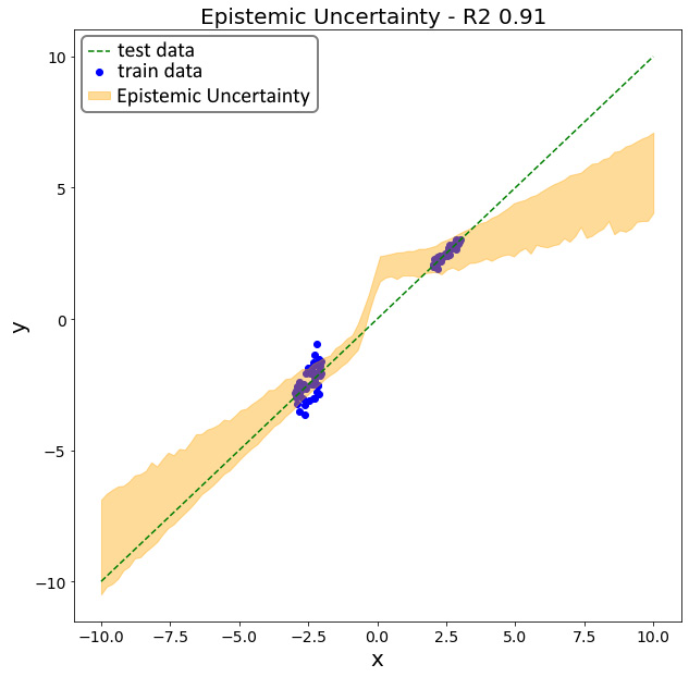
Figure 5.8 – Epistemic uncertainty on test dataset

We can see from the figure that epistemic uncertainty is high in the regions where we do not have sufficient training data. We would like to mention here that, normally, to access epistemic uncertainty one has to build a Bayesian approximation model so that the variations in weight can be captured. One can do it using VariableLayer, available in TensorFlow Probability. However, here, we made use of the fact that dropout layers can act as a Bayesian approximation (Gal and Ghahramani, 2017).

Epistemic uncertainty is a property of the model. Aleatoric uncertainty, on the other hand, is a property of data. There are two types of aleatoric uncertainty. One is homoscedastic uncertainty, where uncertainty is constant and does not change with input. If it is not constant, then we call it heteroscedastic uncertainty. Since heteroscedastic aleatory uncertainty depends on input, we can predict it as a model output. To be able to do that, we can change our loss function to aleatoric loss and instead of a single output tensor, the model outputs a 2D tensor. This enables the model to not just learn the output y, but also its variance. The same can be achieved using the DistributionLambda layer of TensorFlow Probability.

We use the same data as before, and define the heteroscedastic aleatoric loss function (Kendal and Gal, 2017):

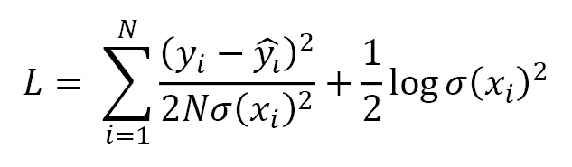
Here, N is the number of data samples, yi is the ground truth, and ŷi is the predicted output. Variance in input is σ2. Now, if you see this function, the first term is a scaled version of the mean square error and ensures that the model predicts close to the ground truth. However, if its predictions are not accurate, the variance term (uncertainty) in the denominator increases to reduce the contribution of the first term. The second term ensures that the model does not go on increasing the uncertainty.

Let us see how regressive uncertainty works:

1. The following Python code implements the preceding loss function:

   # aleatoric loss function
   def aleatoric_loss(y_true, y_pred):
       N = y_true.shape[0]
       se = K.pow((y_true[:,0]-y_pred[:,0]),2)
       inv_std = K.exp(-y_pred[:,1])
       mse = K.mean(inv_std*se)
       reg = K.mean(y_pred[:,1])
       return 0.5*(mse + reg)

   CopyExplain
2. Next, we build the model. Earlier, we had only one neuron in the output layer. Now, we will have two neurons, one corresponding to predicted output y, and the other corresponding to the variance:

   def build_model(layers_shape, input_dim, output_dim):
       inputs = Input(shape=(input_dim,))
       hidden = Dense(layers_shape[0], activation='relu', kernel_regularizer=l2(0.004))(inputs)
       for i in range(len(layers_shape)-1):
           hidden = Dense(layers_shape[i+1], activation='relu', kernel_regularizer=l2(0.004))(hidden)
       outputs = Dense(output_dim)(hidden)
       model = Model(inputs, outputs)
       return model
   model = build_model(layers_shape=[5,10,20,10,5], input_dim= 1, output_dim=2)
   model.summary()

   CopyExplain

Here is the model summary:

Model: "model"
___________________________________________________________
 Layer (type)                Output Shape              Param #
===========================================================
 input_1 (InputLayer)        [(None, 1)]               0
 dense (Dense)               (None, 5)                 10
 dense_1 (Dense)             (None, 10)                60
 dense_2 (Dense)             (None, 20)                220
 dense_3 (Dense)             (None, 10)                210
 dense_4 (Dense)             (None, 5)                 55
 dense_5 (Dense)             (None, 2)                 12
===========================================================
Total params: 567
Trainable params: 567
Non-trainable params: 0
___________________________________________________________

3. Now, to train the model, we need to reshape the data to adjust for the change in the model:

   x_data_reshaped = x_data.reshape(x_data.shape[0], 1)
   y_data_reshaped = np.vstack([y_data, np.zeros(y_data.shape)]).T

   CopyExplain
4. Let us now define the optimizer. We keep it the same as in the first case, rmsprop, and change the loss to our customized loss:

   model.compile(optimizer='rmsprop', loss=aleatoric_loss, metrics=['mae'])

   CopyExplain
5. And finally, train it:

   model.fit(x_data_reshaped, y_data_reshaped,
             batch_size=10, epochs=1000, shuffle=True, verbose=1)

   CopyExplain
6. Let us now plot the aleatoric uncertainty:

   x_test=np.linspace(-10,10,100)
   p = np.array([model.predict(x_test, verbose=0)])
   mean, epistemic_std = np.mean(p[:,:,0], axis=0), np.std(p[:,:,0], axis=0)
   aleatoric_std = np.exp(0.5*np.mean(p[:,:,1], axis=0))
   fig, ax = plt.subplots(1,1,figsize=(10,10))
   ax.scatter(x_data, y_data, s=10, label='train data')
   ax.plot(x_test, x_test, ls='--', label='test data', color='green')
   ax.fill_between(np.squeeze(x_test), np.squeeze(mean+1*aleatoric_std), np.squeeze(mean-1*aleatoric_std),  alpha=0.4, label='Aleatoric Uncertainty (1 SD)', color='orange')
   ax.fill_between(np.squeeze(x_test), np.squeeze(mean+2*aleatoric_std), np.squeeze(mean-2*aleatoric_std),  alpha=0.2, label='Aleatoric Uncertainty (2 SD)', color='blue')
   ax.set_xlabel('x')
   ax.set_ylabel('y')
   ax.set_title('{} - R2 {:.2f}'.format('Aleatoric Uncertainity', r2_score(x_test, mean)))
   ax.legend()

   CopyExplain

The plot for aleatoric uncertainty is as follows:

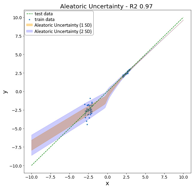
Figure 5.9 – Aleatoric uncertainty on the test dataset

From the figure, we can see that at around -2.5, the aleatoric uncertainty is high, since this was the place in our original training data where there was more noise in the data itself. This type of uncertainty can be problematic for applications where the AI may need to make decisions that can have life-threatening consequences, for example, in the case of a self-driving car. Therefore, there is a need to build models that can not only predict but also score epistemic and aleatory uncertainties while making predictions.

Now that we have seen how to model uncertainty in a regression task, let us move on to quantifying uncertainty in a classification task.

In classification tasks, the standard procedure is to use SoftMax activation in the final layer. This SoftMax activation, by default, already has a measure of confidence (Figure 5.10). However, SoftMax is not very reliable. Consider, for example, a model trained to classify horses and zebras, and it sees a dog; it would not say 50% horse and 50% zebra, instead of assuming it is a black dog. It might think it’s more like a horse, and classify it as a horse with 60% probability.

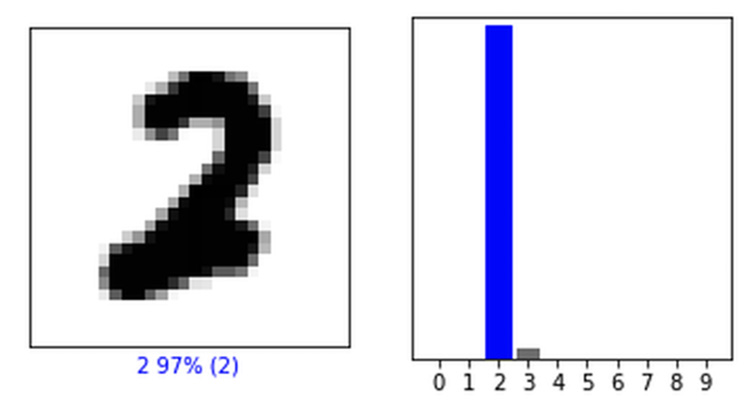
Figure 5.10 – Image from MNIST data and its SoftMax confidence

Mathematically, classification tasks use maximal class probability to determine the class:

Here, K is the total number of classes, and pk is the SoftMax value for class k for that prediction. Some researchers have also tried to use entropy  of the SoftMax prediction. The maximal probability represents a direct representation of certainty, while entropy describes the average level of information in a random variable.

Despite being simple and straightforward to use, these approaches are unreliable, especially when we are dealing with a critical decision AI model such as medical diagnosis.

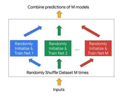
Figure 5.11 – Deep ensemble architecture

One of the ways to quantify uncertainty in classification tasks is by using ensemble methods. Lakshminarayanan et al., show in their paper that using ensemble methods is better than other approaches when the model is presented with out-of-domain data. They trained an ensemble of deep neural networks (Figure 5.11), using the entire MNIST training dataset. The predictions from the trained models were combined as follows:

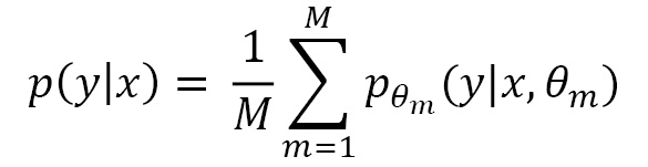
Here, M is the number of ensembled models. In the paper, M=5, y is the prediction for input x, and the θm instances are the network parameters. As you can see, for classification, this corresponds to averaging the prediction probabilities. Additionally, they also generated adversarial examples and performed adversarial training for each network of the ensemble. Figure 5.12, shows the results for the MNIST and NotMNIST datasets:

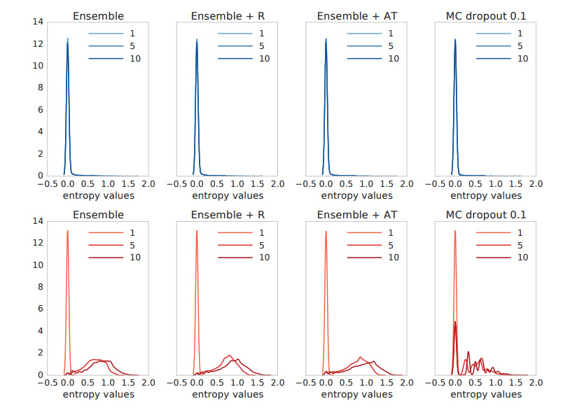
Figure 5.12 – Entropy values for the MNIST dataset (blue) and the NotMNIST dataset (red)

As you can see in the figure, the ensembles work better when presented with the NotMNIST dataset, since the entropy value for NotMNIST spreads over a bigger range and the peak is reduced. They also compared their approach with the Bayesian method (adding Monte Carlo dropout). The figure shows that ensembles give better results. Thus, they showed that deep ensembles generate a low confidence output for out-of-distribution data. In general, for dataset shift and out-of-domain distributions, deep ensembles give consistently better performance when compared to other methods.

A lot of work has been done to quantify uncertainty and create benchmarks for uncertainty and robustness. In this section, we will cover some of the prominent ones. Please remember that the standards are still in the nascent stage, and as a result, many of these tools and GitHub repos may have certain limitations.

The Uncertainty Baselines library

Developed by researchers from the Google Brain research team, the University of Oxford, the University of Cambridge, Harvard University, and the University of Texas, the Uncertainty Baselines library contains a set of baselines that you can use to compare the performance of different deep learning methods. The baselines are implemented using high-quality methods, and they are available for a variety of tasks. You can use these baselines to get started with your own experiments. The complete work is accessible via the GitHub repo at https://github.com/google/uncertainty-baselines.

At present, there is no stable version. However, users can install it and experiment directly via Git. The library aims to provide users with a modular, framework-agnostic, hardware-agnostic tool.

Keras-Uncertainty

Keras-Uncertainty is a high-level API that can be used to measure how trustworthy a ML model’s predictions are. This is important for many real-world applications, where you not only need to know what the model predicts but also how confident we should be in its predictions. The library is available at https://github.com/mvaldenegro/keras-uncertainty. Figure 5.13 shows the uncertainty for a classification task using Keras-Uncertainty. For demonstration, we used the make_moon method from scikit-learn to create synthetic classification data. We trained five models and plotted the respective uncertainty using the Keras-Uncertainty library.

Figure 5.13 – Uncertainty for binary classification problem

Robustness metrics

Developed by Google Research, the Robustness Metrics library provides functions and methods that can help in the evaluation of classification models. It defines three sets of metrics:

• Out-of-distribution generalization: This measure assesses the model’s ability to accurately classify objects that share similarities but may have varying perspectives.
• Stability: This measure evaluates the stability of predictions made by the model when there are changes in the input, and how effectively the model performs with natural disturbances.
• Uncertainty: This measure gauges the proximity of the probabilities estimated by a model to the actual probabilities.

The Robustness Metrics library can be used even for non-vision models. Essentially, if you have a classification task, you can try this library. It depends on TensorFlow and TensorFlow Probability, therefore, before you use it you should install them on your system.

This chapter started by introducing the different components of ML pipelines. Then we discussed various ML tasks and different algorithms that are used for those tasks.

The main theme of the chapter was uncertainty in deep learning. This uncertainty can be due to the data or the model – or both. We discussed the two types of uncertainty, aleatory and epistemic. The chapter also discussed various methods that have been used in the literature to quantify uncertainty. It also delved deep into the causes of uncertainty. Next, we implemented algorithms to quantify uncertainty in regression tasks. Finally, the chapter discussed the methods used to quantify uncertainty in classification tasks. There is a need to develop baselines and benchmarks for uncertainty and robustness in deep learning. A lot of work is taking place in this area; however, uncertainty and robustness are still critical research problems in AI and ML.

In the next chapter, we will delve into the concept of hyperparameters, and how to use AutoML and MLOps to streamline your ML workflow.

• Efficientnet: Rethinking model scaling for convolutional neural networks. In International conference on ML, Tan, M., & Le, Q. (2019, May). (pp. 6105-6114). PMLR. http://proceedings.mlr.press/v97/tan19a/tan19a.pdf)
• Uncertainty characterization in risk analysis for decision-making practice, Zio, E., & Pedroni, N. (2012). FonCSI. https://www.researchgate.net/publication/266391086_Uncertainty_characterization_in_risk_analysis_for_decision-making_practice
• Attention is all you need. Advances in neural information processing systems, Vaswani, A., Shazeer, N., Parmar, N., Uszkoreit, J., Jones, L., Gomez, A. N., … & Polosukhin, I. (2017). 30. https://proceedings.neurips.cc/paper/2017/file/3f5ee243547dee91fbd053c1c4a845aa-Paper.pdf
• Dropout as a Bayesian approximation: Representing model uncertainty in deep learning. In International conference on ML, Gal, Y., & Ghahramani, Z. (2016, June). (pp. 1050-1059). PMLR. http://proceedings.mlr.press/v48/gal16.pdf
• What uncertainties do we need in Bayesian deep learning for computer vision? In Advances in neural information processing systems, Kendall, A., & Gal, Y. (2017). 30. https://arxiv.org/pdf/1703.04977.pdf
• A survey of uncertainty in deep neural networks, Gawlikowski, J., Tassi, C. R. N., Ali, M., Lee, J., Humt, M., Feng, J., … & Zhu, X. X. (2021). arXiv preprint arXiv:2107.03342. https://arxiv.org/pdf/2107.03342.pdf
• A review of uncertainty quantification in deep learning: Techniques, applications and challenges, Abdar, M., Pourpanah, F., Hussain, S., Rezazadegan, D., Liu, L., Ghavamzadeh, M., … & Nahavandi, S. (2021). In Information Fusion, 76, 243-297. https://arxiv.org/pdf/2011.06225.pdf
• Simple and scalable predictive uncertainty estimation using deep ensembles. In Advances in neural information processing systems, Lakshminarayanan, B., Pritzel, A., & Blundell, C. (2017). 30. https://arxiv.org/pdf/1612.01474.pdf
• Robustness Metrics, J. Djolonga, F. Hubis, M. Minderer, Z. Nado, J. Nixon, R. Romijnders, D. Tran, and M. Lucic. 2020. https://github.com/google-research/robustness_metrics
• Uncertainty Baselines: Benchmarks for uncertainty & robustness in deep learning, Nado, Z., Band, N., Collier, M., Djolonga, J., Dusenberry, M. W., Farquhar, S., … & Tran, D. (2021). arXiv preprint arXiv:2106.04015. https://arxiv.org/pdf/2106.04015
• On robustness and transferability of convolutional neural networks, Djolonga, J., Yung, J., Tschannen, M., Romijnders, R., Beyer, L., Kolesnikov, A., … & Lucic, M. (2021). In Proceedings of the IEEE/CVF Conference on Computer Vision and Pattern Recognition (pp. 16458-16468). https://arxiv.org/pdf/2007.08558.pdf