Machine Learning (ML) has made massive strides in recent years, with applications in everything from finance to healthcare. However, these systems can often be opaque and biased against certain groups of people. In order for ML to live up to its potential, we must ensure that it is fair and unbiased.

In Chapter 7, we discussed the concept of fairness in the context of data generation. In this chapter, we will cover different optimization constraints and techniques that are essential to optimizing and obtaining fair ML models. The focus of this chapter is to enlighten you about new custom optimizers, unveiled by research that can serve to build fair supervised, unsupervised, and semi-supervised ML models. In a broader sense, you will learn the foundational steps to create and define model constraints that can be used by different optimizers during the training process. You will also gain an understanding of how to evaluate such constraint-based models with proper metrics, and the extra training overheads incurred when employing the optimization techniques, which will enable you to design your own algorithms.

In this chapter, the following topics will be covered:

• The concept of fairness as applied to ML
• Explicit and implicit mitigation of fairness issues
• Fairness constraints for a classification task
• Fairness constraints for a regression task
• Fairness constraints for a clustering task
• Fairness constraints in reinforcement learning
• Fairness constraints for a recommendation task
• Challenges of fairness

This chapter requires you to have Python 3.8 along with some Python packages:

• TensorFlow 2.7.0
• NumPy
• Matplotlib

Fairness is a subjective term. It has different meanings depending on culture, time, race, and so on. We could write endlessly on the topic of fairness in society; however, in this chapter, our focus is fairness with respect to ML. In Chapter 7, you became familiar with the concept of fairness and how data plays an important role in the fairness of your ML model. In this chapter, we will expand on the concept of fairness.

As you might have already realized, fairness does not have a universal definition. For example, seen from the point of view of an organization, fairness can have three different dimensions (Cropanzano et al., 2001. See Further reading):

• Distributive fairness: The algorithm should be fair in allocating important resources, for example, in hiring.
• Interactional fairness: The algorithm should be able to explain the rationale behind it, and the explanation provided by the algorithm should be perceived as fair by the people concerned, for example, why A should get a promotion over B.
• Procedural fairness: The algorithm should not generate different results when used for different subgroups within an organization, for example, different recommendations for women than for men. If it does, it should be because of explainable societal or biological reasons.

These are demonstrated in Figure 8.1.

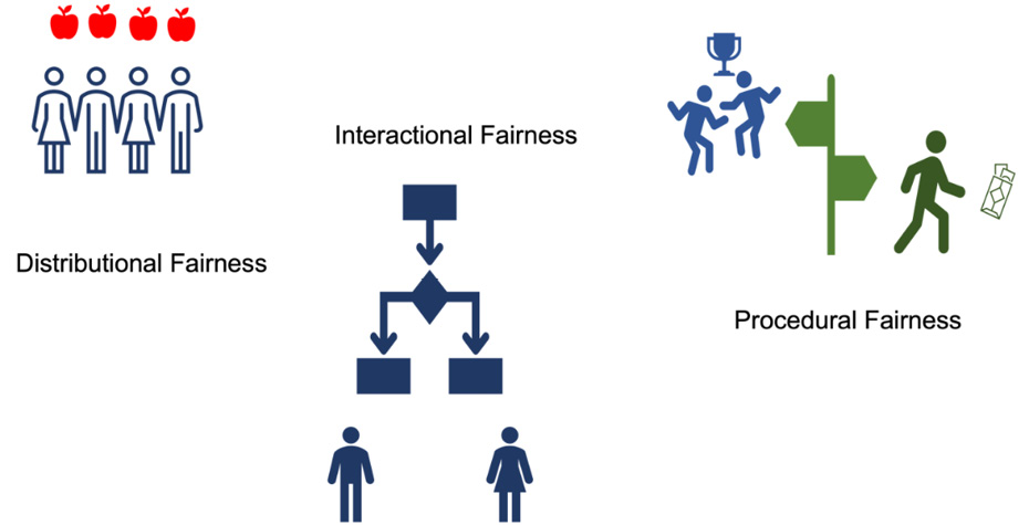
Figure 8.1 – Different dimensions of fairness in an organization

Bias and fairness are two terms that are often used interchangeably in the ML community. However, we feel that they should be differentiated. Taking a leaf out of Booth’s book (https://dl.acm.org/doi/fullHtml/10.1145/3462244.3479897), we define bias as a systematic error that alters the model’s decision based on specific input information (such as gender and geographical location). Often called measurement bias, this bias arises either because unnecessary information is added to an input feature space (construct contamination) or because the model is not capturing all the aspects of what you are measuring (construct deficiency). Here, construct refers to features that cannot be directly measured, and instead need to be inferred from measurements. Figure 8.2 shows different sources of bias.

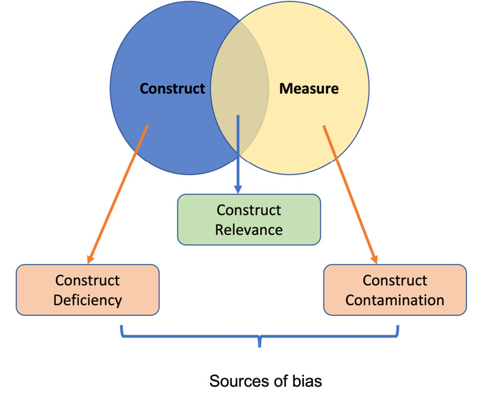
Figure 8.2 – Sources of measurement (adapted from Booth et al., 2021)

A biased model may not always be a bad thing – it is possible for a model to be biased but fair (Figure 8.3). As illustrated in the paper Algorithmic Fairness, by Pessach et al., it is possible for a model to consider both SAT scores and demographics for the admission selection process and allocate seats unequally to students based on whether they come from a privileged background or an unprivileged background, favoring those from underprivileged backgrounds. While such a model is biased, it is fair because a student from an underprivileged background will have had to overcome many more challenges to achieve that score and probably has higher potential.

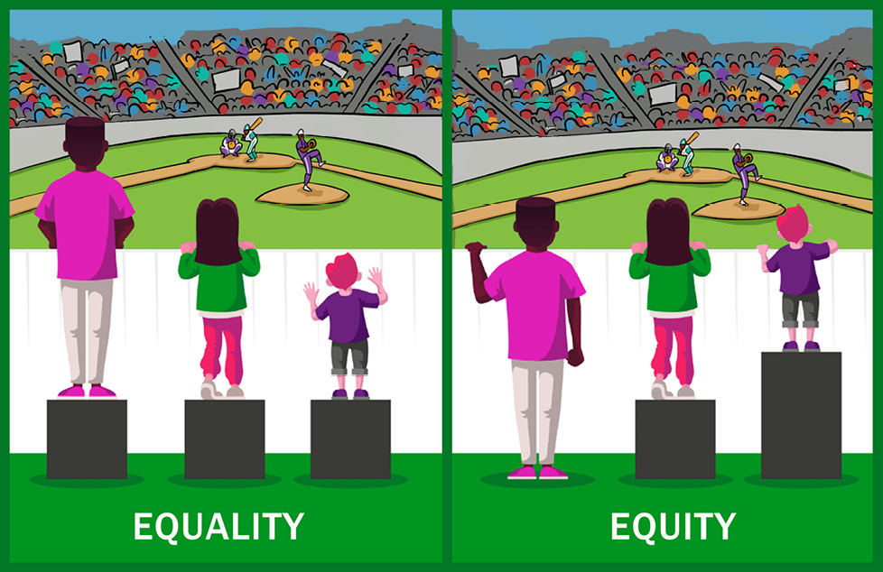
Figure 8.3 – Biased resource allocation to candidates based on their demographics and so on can result in a fair algorithm by giving tools to the underrepresented classes of society

Now that we have set the boundaries between fairness and bias, we will proceed to look at unfairness and methods to mitigate unfairness.

In recent years, researchers have developed various techniques to mitigate unfairness in AI models. These methods can be applied at different stages of model development:

• Preprocessing: Preprocessing methods work by adjusting the training data distribution so that the sensitive groups are balanced.
• Postprocessing: Postprocessing methods work by calibrating the predictions after the model has been trained.
• In-processing: These methods incorporate fairness directly into the model design.

In Chapter 7, we discussed preprocessing methods and techniques. In this chapter, we will discuss in-processing unfairness mitigation methods first, and later discuss different fairness constraints as applied to different ML tasks.

In-processing methods

Using in-processing methods offers certain benefits:

• It has been observed that ML models often amplify the bias present in data. Using in-processing techniques for unfairness mitigation can help in addressing this problem. This is because the problem of amplification is caused by the algorithm, and since in-processing methods take fairness into consideration alongside model optimization it can help reduce or eliminate the issue.
• Fine-tuning pre-trained models has become a popular approach to customize modeling for different tasks with limited training data. Although transfer learning from pre-trained models has alleviated the need for large amounts of training data, the issue of bias in pre-trained models has become more critical as the pre-trained models are usually trained on biased data. By using techniques such as contrastive learning, it is possible to use in-processing methods to mitigate unfairness in pre-trained models.

Developing efficient in-processing methods is still a challenge. Existing algorithms are not sufficient, and we need to focus on developing new methods that can address fairness issues when sensitive attributes are not disclosed or available.

In-processing unfairness mitigation methods can be further subdivided into two: implicit methods and explicit methods. In explicit methods, unfairness mitigation is achieved by incorporating the fairness metrics within the objective function using either fairness constraints or regularization parameters. Implicit methods, on the other hand, rely on modifying learning strategies of the deep learning model – for example, by including adversarial examples while training. Explicit methods are easy to implement and are often flexible. Let us now explore the ways to mitigate unfairness with the help of explicit methods.

Note

In Chapter 7, we covered many fairness measurement metrics. In this chapter, we will call an algorithm fair if it is able to achieve good results for the fairness metrics it is designed for.

In the rest of the chapter, we will discuss various techniques for unfairness mitigation. Specifically, we will tackle two specific fairness issues:

• Disparate treatment: Disparate treatment is when there is a difference in the ways individuals are treated based on their race, gender, or other protected characteristics. For example, if an algorithm is trained on data that is mostly about males, it may predict a higher salary rise for a male candidate and a lower salary rise for a female candidate despite them having the same number of years of experience. Most often, disparate treatment arises from biased data, or using sensitive information while training the model.

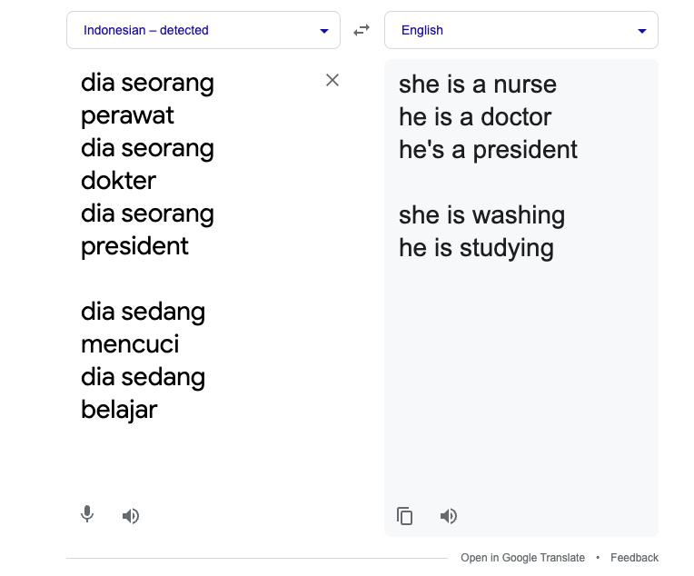
Figure 8.4 – Example of disparate treatment by Google’s translate algorithm (adopted from Fitria, 2021)

• Disparate impact: Disparate impact is when the model treats certain groups differently, even when the model is not explicitly trained on corresponding sensitive attributes. For example, if an algorithm is trained on data that is mostly male, it may learn to associate male names with high-status jobs and female names with low-status jobs. This can happen when unknowingly, the model creates some proxy attributes that correlate with sensitive information.

As discussed in the previous section, explicit unfairness mitigation is achieved by adding regularizers or by including constraints within the loss function. In this section, we will expand on the explicit unfairness mitigation techniques and explore some of the recently proposed strategies for this.

Fairness constraints for a classification task

Let us first build an understanding of classification tasks in ML. Consider Y, X, and S to be random variables, corresponding to the class/label, non-sensitive input features, and sensitive input features, respectively. Our training dataset, D, will then consist of instances of these random variables:

D = { (y, x, s) }

The aim of the classification task is to find a model, M, defined by parameters, Θ, such that it is able to correctly predict the conditional probability of a class when sensitive and non-sensitive features are given, M[Y|X,S; Θ]. The model parameters are estimated by using the Maximum Likelihood Estimator (MLE):

Let us see how we can modify this loss function to mitigate unfairness.

Adding a prejudice removal regularizer

The paper Fairness-Aware Classifier with Prejudice Remover Regularizer, by Kamishima et al., introduced a prejudice removal regularizer term to the loss function, as shown in the following figure:

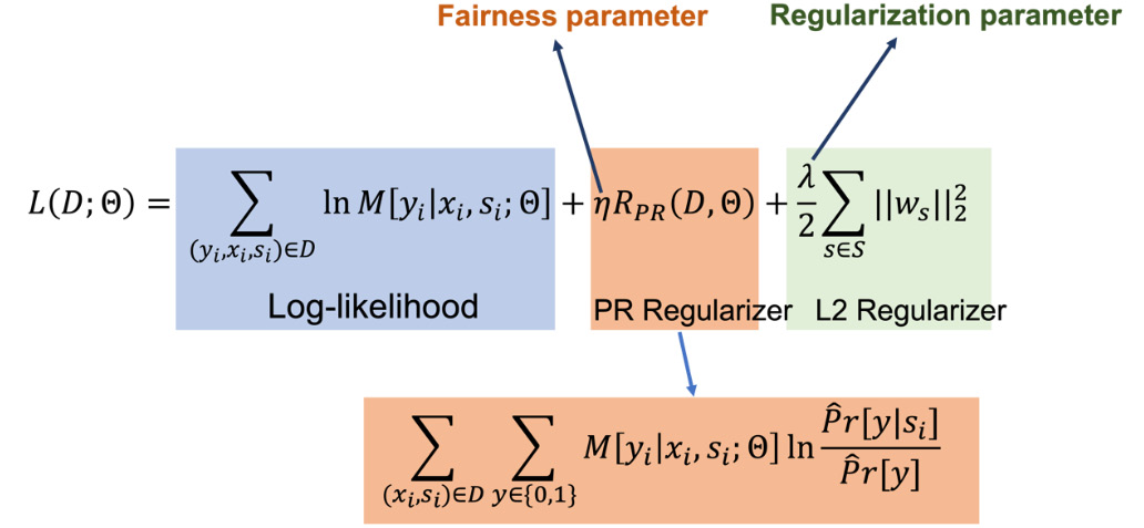
Figure 8.5 – Adding a prejudice removal regularizer term to the loss function

To measure the model fairness, Calder’s and Verwer’s 2 Naïve Bayes (CV2NB) score is used. In the NNabla Examples library, the util module contains the CVS function for calculating the score. To have a point of comparison, it is good to first build a simple classifier:

1. To begin, we create a function to create a simple four-layered neural network classifier. Between each layer, we have added dropout layers for regularization to avoid overfitting:

   def Classifier(n_features, n_hidden=32, p_dropout=0.2,train=True):
       with nn.parameter_scope('classifier'):
           layer1 = PF.affine(n_features, n_hidden, name='layer1')
           layer1 = F.relu(layer1)
           if (train):
               layer1 = F.dropout(layer1,p_dropout)
           layer2 = PF.affine(layer1, n_hidden, name='layer2')
           layer2 = F.relu(layer2)
           if (train):
               layer2 = F.dropout(layer2,p_dropout)
           layer3 = PF.affine(layer2, n_hidden, name='layer3')
           layer3 = F.relu(layer3)
           if (train):
               layer3 = F.dropout(layer3,p_dropout)
           layer4 = PF.affine(layer3, 1, name='layer4')
       return layer4

   CopyExplain

The preceding code makes use of the NNabla (imported as nn) library to build the network.

2. Now, if we create a simple classifier using the previous function and train it on the Adult dataset (https://archive.ics.uci.edu/ml/datasets/Adult), the result shows the accuracy and CV2NB score:

   Classifier accuracy :  84.85797101449275 Classifier CV2NB Score : 0.1644

   CopyExplain
3. But now, if you include the prejudice removal regularizer term and retrain the same classifier with the modified loss function, you can see that the CV2NB score improves:

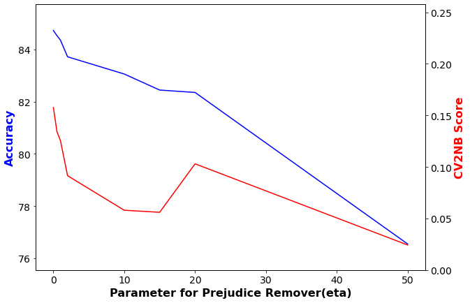
Figure 8.6 – Accuracy versus CV2NB score on adult dataset after adding prejudice removal regularizer term to the loss function

In the preceding figure, we can see that as η (the fairness parameter) increases, the CV2NB score also improves. The larger value of the fairness parameter enforces fairness. However, we can see that the cost of increased fairness is accuracy; a balance must be reached between the two. Also, you can see that a classifier with the prejudice removal regularizer had a CV2NB score of 0.16, which is higher compared to a classifier trained without using the prejudice removal regularizer (Figure 8.6), thus proving that adding the regularizer creates a more fair model.

Modifying the objective

A great deal of work in this area has been done by M. B. Zafar. Those interested in his complete work can refer to his GitHub repo: https://github.com/mbilalzafar/fair-classification. We will consider two different classifiers: support vector machines and logistic regressors. The common thing between these classifiers is that both are based on finding a decision boundary that separates the classes. In support vector machines, the decision boundary is found by maximizing the distance between minimum support vectors, and in logistic regressors, the decision boundary is found by minimizing the log-loss function.

For simplicity, we consider the case of a binary classifier. For a linear binary classifier, the decision boundary is defined as follows:

ΘTX = 0

Here, Θ refers to the coefficients of the hyperplane defining the decision boundary.

For this to work, fairness against disparate treatment is ensured by making sure that sensitive attributes (S) are not used in decision-making/prediction. Continuing with our approach, this means that S ∩ X = ∅; that is, they are disjointed.

For disparate impact, the 80% rule (more generally called the p-rule) is used as the fairness metric. Translating the 80% rule to the distance boundary, it means that if dθ(x) is the signed (or oriented) distance of feature vector x from the decision boundary, then the ratio of users with a specific sensitive feature having a positive signed distance and users without the sensitive feature having a positive signed distance is no less than 80:100. Mathematically, for a binary sensitive attribute, s ∈ {0,1}, we can express the p-rule as follows:

To mitigate the unfairness, Zafar et al. introduced the concept of decision boundary covariance. They defined it as the covariance between the user’s sensitive features and the signed distance of the user’s input features to the decision boundary. Mathematically, it would be as follows:

Simplified, this expression is reduced to the following:

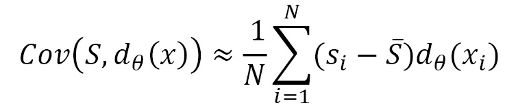
It is easy to include this in the classifier objective since this is a convex function. Let us put it into action. We created a synthetic dataset with two sensitive features and one non-sensitive feature. The following graph shows the generated data points.

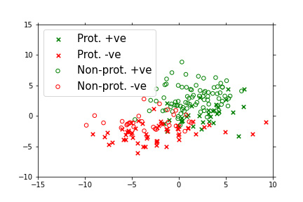
Figure 8.7 – Synthetic data generated with two sensitive features and one non-sensitive feature (showing only 200 sample points)

The details of the data generated by us are as follows:

Total data points: 4000
# non-protected examples: 1873
# protected examples: 2127
Non-protected in positive class: 1323 (71%)
Protected in positive class: 677 (32%)

If we do not use any fairness constraints and train a simple classifier, the accuracy that we get is 87%, but the classifier follows only a 41% p-rule, as opposed to the desired 80%. Now, there are two strategies we can adopt:

• Maximize accuracy under fairness constraints: In this case, the constraints are put so that the p-rule is satisfied while maximizing the accuracy of the classifier. This is achieved by the following:

Minimize L(D,Θ) subject to 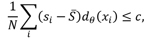 and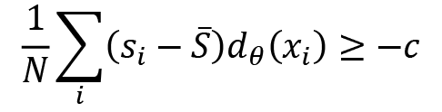 

Here, c refers to the covariance threshold. It specifies an upper bound on the covariance between sensitive features and the signed distance of the input features from the decision boundary. The covariance threshold provides a trade-off between accuracy and fairness.

As c decreases (c → 0), the classifier becomes fairer at the cost of accuracy. The following is the result of the classifier trained using the fairness constraints.

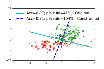
Figure 8.8 – Decision boundary of an unconstrained and constrained logistic classifier when trained on the synthetic data

You can see that the accuracy of the classifier reduced slightly (71%), but the p-rule value is 104% – this means the classifier is fair. The protected versus non-protected ratio in the positive class is 53:51. The graph also shows the decision boundary for the original and constrained classifiers.

• Maximize fairness under accuracy constraints: In this case, we minimize the covariance decision boundary, subject to the constraint that the loss of the constrained classifier (L(D,Θ)) is less than the loss of the unconstrained classifier (L(D,Θ*)) – in other terms, the following:

Minimize 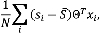 subject to .

Here, Li represents loss associated with the i-th user in the training set. The following graph shows the results obtained using these constraints.

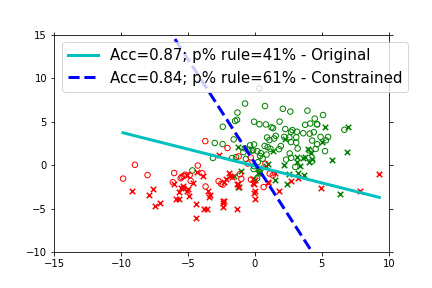
Figure 8.9 – Decision boundary of an unconstrained and constrained logistic classifier when trained on the synthetic data

We can see that now, while the p-rule has improved from 41% to 61%, the decrease in accuracy is not very significant. For businesses, this is important. You cannot launch a product that is fair but not accurate.

The preceding graphs were generated using the code provided by the Kamishima group with the following parameters:

n_samples = 2000 # Number of data points
disc_factor = math.pi / 4.0 # represents f in the paper-- decrease it to generate more discrimination
gamma = 2000.0

This approach helps mitigate the disparate impact on classification tasks. The approach can be extended to many classification tasks.

Fairness constraints for a regression task

In regression, the task changes from finding a decision boundary to finding a hyperplane that contains most of the data points. A classifier is good when the decision space is small and discrete, but more often, decision spaces are continuous. For example, instead of telling whether a person will default on a loan or not (a binary world), it is more useful for decision-makers to know the probability of a person defaulting on a loan (a continuous value between 0 and 1). In these scenarios, regression is a better option. The major difference is that while in the case of classification the logit loss function is used, in the case of regression, the loss function is conventionally the Mean Square Error (MSE). This means that we can add a regularizer term, just as we did with the classifier, to get a fair regression. Indeed, this was attempted by Berk et al., and they proposed a general framework for fairness in both regression and classification tasks:

Here, L is the conventional loss function (for the classifier, the conventional loss is logit loss, and for regression, we conventionally use the MSE loss). They added a λ -weighted fairness loss term, fp. To take care of overfitting, there is the standard L2 regularization term. This method can be applied to any model with a convex optimization function.

Using this approach, they were able to achieve both individual and group fairness. Let us see how.

Individual fairness using a fairness penalty term

Continuing with our previous terminology, let s be a binary sensitive feature, s ∈ {0,1}. It tells us whether a user belongs to the sensitive group or not. Then, for individual fairness, the penalty term is defined as follows:

Here, d is a non-negative function, which is a measure of the absolute difference between the outputs for sensitive and non-sensitive groups (|yi – yj|), n1 is the number of individuals belonging to the sensitive group, and n2 is the number of individuals not belonging to the sensitive group.

We can see that every time the model treats the inputs corresponding to sensitive and non-sensitive differently, it is penalized.

Group fairness using a fairness penalty term

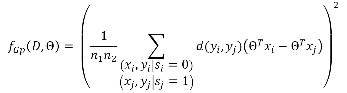
Now, for group fairness, we would like, on average, for the two group samples to have similar predictions. This is achieved by defining the fairness penalty term as follows:

Now, to verify whether it really works for the regression case, we make use of the communities and crime dataset, available from the UCI ML repository (http://archive.ics.uci.edu/ml). The dataset contains features related to per-capita violent crime rates in different communities across the US. Here, the sensitive feature is the race of the individual and the task is to predict the crime rate.

Figure 8.10 shows fairness loss versus MSE loss for the dataset. Here, single refers to the case where only one model is built for the two sensitive groups and separate refers to where we have separate models.

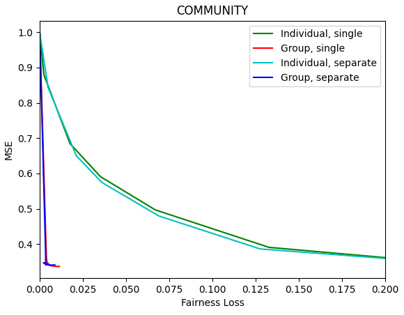
Figure 8.10 – MSE loss versus fairness for the communities and crime dataset

We can see once again that there is a price to be paid for fairness in terms of accuracy. Thus, care must be taken by model builders when defining the type of fairness they care about, making a decision specific to their application, and they should decide on a proper balance between prediction accuracy and fairness.

Fairness constraints for a clustering task

A clustering task involves grouping the given data points into clusters. Although there are supervised clustering algorithms, unsupervised clustering is more common. Here, the data points X = {xp ∈ RM,p = 1, … , N} are provided and the task is to assign them to K clusters. Let M be the cluster assignment vector: M = [m1, … , mN ] ∈ [0,1]NK. Now, say the data contains sensitive information, for example, J for different demographic groups. We can represent the sensitive information as a vector, Sj = [sj, p] ∈ {0,1}N , so if point p is assigned to group j, then sj, p = 1; otherwise, it is 0.

One of the most widely used clustering algorithms, K-means, clusters the given data points in K clusters by minimizing the sum of the distance between individual data points and the representative cluster centroids. We can add a fairness penalty. In the paper Variational Fair Clustering, the authors added the Kullback-Leibler divergence term between the required demographic proportions and the marginal probability (Pm=[P(j|m)]) of the demographics within cluster m. In terms of the cluster assignment vector and demographic information vector, the marginal probability can be expressed as follows:

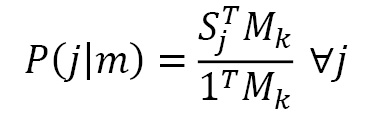
The T here denotes the mathematical transpose operator. The modified objective function is shown in the following figure:

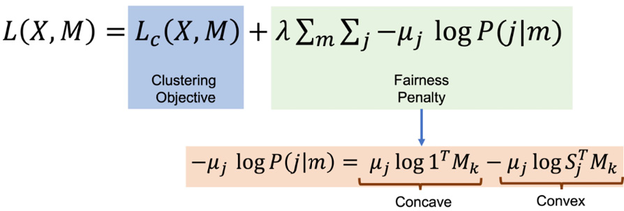
Figure 8.11 – Loss function with a fairness penalty for the clustering task

The interesting thing to note is that the fairness penalty is represented by a cross-entropy term between the required demographic proportion, U, and the respective marginal probability, Pk. This penalty can further be decomposed into two parts, one convex and the other concave. You are encouraged to read the original paper for complete mathematical proofs of bounds, convergence, and monotonicity guarantees (https://arxiv.org/abs/1906.08207).

Table 8.1 lists the results of applying these fairness constraints on different datasets. The synthetic datasets are created according to the demographic breakdown; both are created with 450 data points and two demographic groups. In the synthetic dataset, both groups have an equal number of required proportions generated; however, in synthetic unequal, we created 310 and 140 data points for the two demographic groups:

Table 8.1 – Table listing clustering objective, fairness error, and average balance on different datasets using K-means clustering with a fairness penalty

Figure 8.12 shows the clusters obtained on the synthetic and synthetic unequal datasets by applying K-means with a fairness penalty.

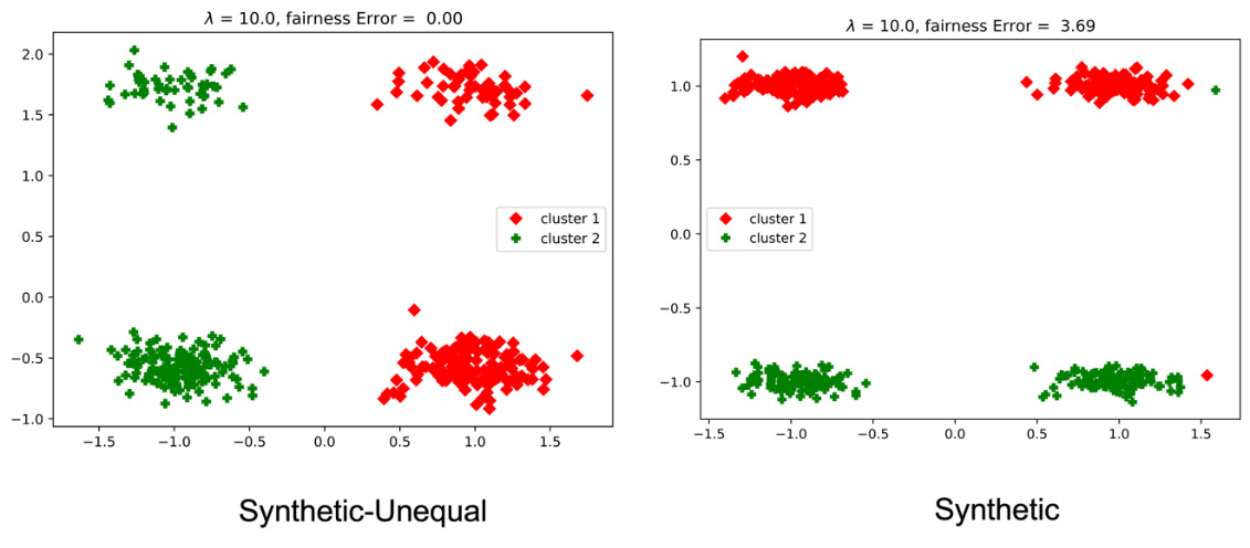
Figure 8.12 – Clusters on the two datasets using K-means with a fairness penalty

The same approach can also be applied to the K-median clustering algorithm and the Ncut clustering algorithm.

Fairness constraints for a reinforcement learning task

Reinforcement learning is quite different from the supervised learning used in regression and classification tasks and the unsupervised learning used in the task of clustering. What makes it different is that here, the algorithm has no idea of the desired output. Every choice it makes affects not only its present learning but also future outcomes. In reinforcement learning, the algorithm gets feedback from the environment; it is this feedback that helps it learn.

To define the reinforcement learning task, we can say that the system consists of the agent (reinforcement learning agent or algorithm) and an environment. The agent can perceive the environment through state vectors, s, it can bring changes in the environment through actions, a, and the environment may give the agent feedback in terms of reward, r (Figure 8.13). The goal of the agent is to find the optimal policy, π(s,a), that will maximize the rewards.

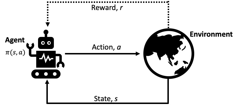
Figure 8.13 – Reinforcement learning framework

We can represent a simple reinforcement learning problem as a multi-armed bandit problem. The problem imagines a gambler playing at a row of slot machines. They have to decide the order in which the slot arms will be played so as to maximize their rewards. We can define the problem as having N slots, with the task of the gambler to choose one arm at each time step, t:

At each time step, t, the gambler receives a reward, rt ∈ [0, 1]N, decided by a fixed distribution, E[rt(it)] = μ(it). However, the gambler is not aware of this distribution. The only thing they can observe is the reward, rt(it). The goal of the gambler is to choose the arms in a sequence that maximizes the total reward:

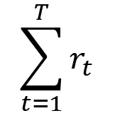
The optimal reward probability of best the optimal slot arm is as follows:

 where, 

To train our agent to play the role of the gambler, we can define our loss function as a regret function – representing the regret that the agent will have by not selecting the optimal slot arm at time step t:

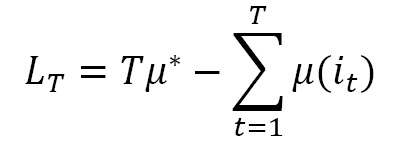
We can think of the multi-armed problem as a resource allocation problem – there are limited resources and they should be allocated for maximum performance. When the reinforcement learning agent starts, it has no idea what action would result in a good reward, and therefore most reinforcement learning agents use the technique called exploration and exploitation. The idea is that the agent initially explores all the possible actions by choosing random actions, learns from them (exploration), and later, when sufficient experience is gained, uses the action as guided by the learned policy (exploitation). One of the algorithms used to implement exploration/exploitation is the ε greedy algorithm (Mnih, 2015).

There is always a trade-off between exploration and exploitation. In the ɛ greedy algorithm, the balance between exploration and exploitation is achieved by decreasing the exploration parameter, ɛ. Another way to achieve the balance between exploration and exploitation is using the Upper Confidence Bound (UCB). The UCB algorithm works by maintaining an estimate of the expected reward for each action. At each step, the algorithm selects the action with the highest estimated reward. However, the UCB algorithm also adds a term to each estimate that encourages exploration. This term is based on the uncertainty of the estimate, and it increases as the number of times an action has been taken decreases. As a result, the UCB algorithm strikes a balance between exploration and exploitation, and it often outperforms other algorithms in online settings.

In this section, we will apply fairness constraints to the multi-armed bandit-based resource allocation problem. The intention is to introduce the notion of fairness to resource distribution. Today, AI-based programs are making decisions in allocating resources such as medical care, loans, and subsidies. Can we ensure fairness in this distribution? Also, does fairness in distribution have an effect on collaboration?

One approach to deal with this issue was given by Claure et al. in the paper Multi-Armed Bandits with Fairness Constraints for Distributing Resources to Human Teammates. They put fair-use constraint limits on the number of times an individual may be assigned a resource, ensuring that all users get what they require. They modified the unconstrained UCB algorithm so as to estimate the expected reward of each arm by using the mean of its empirical rewards in the past and how often it has been pulled.

To evaluate their method, they considered the environment of a collaborative Tetris game, pairing teams of two people with the task of completing a game of Tetris together using their algorithm. The algorithm would decide at each time step which of the two players has control over the falling piece. They later asked the participants to describe whether they felt that the algorithm gave them turns fairly or not: that is their perception of the game’s fairness.

The following table shows the participants’ perception for different constraint limits:

Table 8.1 – Participants’ perception in the experiment for different constraint limits

Their work shows that using their variation of the algorithm, it is possible to allocate resources fairly. This leads to higher trust among individuals without any decrease in performance.

Fairness constraints for recommendation systems

Recommender systems are used to make suggestions for products, services, potential friends, or content. They rely on feedback data and typically run using an ML algorithm. For example, an online bookstore may use a recommender system to classify books by genre and suggest similar books to customers who have purchased a book. Facebook uses a recommender system to suggest potential friends to users. YouTube uses a recommender system to suggest related videos to users who are watching a video. Generally, recommender systems are used to solve the cold-start problem, where it is difficult to make suggestions for new users or items with little data.

Recommender systems are classified into three types based on the information on which they are based: collaborative, content-based, and hybrid filtering. Collaborative filtering recommender systems rely on the collective intelligence of the community to make recommendations. Content-based recommender systems use information about the items themselves to make recommendations. Hybrid recommender systems combine both collaborative and content-based approaches to make recommendations. Each of these approaches has its own strengths and weaknesses, and the best recommender system for a particular application will depend on the specific requirements.

In recent years, recommender systems have become increasingly prevalent in many aspects of our lives. From online shopping to social media, these systems play a key role in helping us find the products, services, and content that we are looking for. However, these systems are not perfect. In particular, they can often suffer from a variety of biases that can lead to unfair recommendations. For example, a recommender system may inadvertently favor certain groups of users over others. This can result in unusable recommendations for some users and can even lead to discriminatory behavior. Therefore, it is essential to address the potential for unfairness in recommender systems. Fortunately, there has been recent progress in this area, and there are now a number of methods that can help to mitigate the problem. With continued research, there is the potential for recommender systems to be made more fair and inclusive for all users.

Recommender systems are multi-stake platforms, with three stakeholders: consumers, the supplier, and the platform:

• Consumers are the users of the platform. They come for suggestions. They use the platform because they might be searching for something or having difficulty in deciding, say, in what to buy. They anticipate that the platform will provide a fair and objective suggestion.
• Suppliers or providers are on the other side of the recommender system. They provide the service and, in return, gain some utility from the consumers.
• Finally, there is the platform itself. It brings consumers and providers together and makes some benefit from it.

Therefore, when we talk of fairness in recommender systems, we also need to clarify which type of fairness we are talking about. In general, we talk of two types of fairness, that is, provider fairness and consumer fairness:

• Provider fairness is concerned with the items that are being ranked or recommended. Here, the notion of fairness is that similar items or groups of items should be ranked or recommended in a similar way. As an example, consider two articles about the same subject. If one is ranked higher because it has more views, this would be unfair because it is giving more weight to popularity instead of quality. To fix this, the algorithm could look at other factors, such as recency, number of shares, and number of likes, to get a more accurate idea of quality. By taking these factors into account, the algorithm would be fairer to both articles.
• Consumer fairness has a focus on the users who receive or use the data or service. A fair recommendation algorithm, in this case, would ensure that users or groups of users receive the same recommendations or rankings. Continuing with the example of the recommender system suggesting articles, if two readers have the same educational background and interest, the algorithm should recommend the same/similar articles to them, without considering sensitive attributes such as gender or age.

One approach to achieving fairness in recommendation systems is to treat them as classification algorithms, with recommendation being a class. Another way is to treat recommendation systems as a ranking problem; here, the recommendation is a ranked list, L. We have already covered how fairness constraints can be added to classification tasks. In this section, we will discuss fairness constraints in ranking, based on the approach developed in the paper Ranking with Fairness Constraints by Celis et al. The basic idea is to put constraints on the number of items that can appear in the top k places from different groups.

Let us start with defining the ranking problem. We have m items, and the goal is to output a list of n items (n ≪ m) in an order that is most valuable to a consumer or provider. We define a number, Wij, that captures the value that an item, i, i ∈ [m], contributes if placed at rank j. There is more than one way to get the value of Wij. We can define it as a ranking maximization problem. Here, the task is to assign each item a position such that the total value is maximized.

To ensure fairness, Celis et al. added constraints in the form of upper (Ul,k) and lower (Ll,k) bounds on the number of objects with property l that are allowed to appear in the top k position of the ranking. We can represent the position of items via a binary matrix, x, which would be an nxm matrix. The xij element of this binary matrix tells us whether the i-th item is ranked at the j-th position. The constraints are put on the matrix:

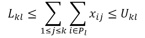
Here, {1, 2, … , p} is the set of properties, and Pl ⊑ [m] represents the set of items with property l. With this change, the ranking maximization will become the following:

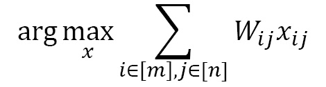
This is illustrated in the following figure:

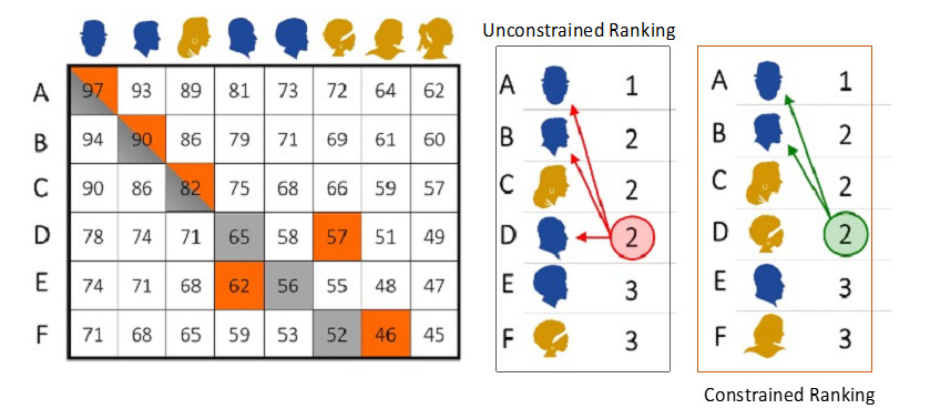
Figure 8.14 – A sample matrix of W. The values represent the optimal unconstrained ranking (gray) and constrained ranking (orange). There is an upper constraint of 2 on the number of males in the top six positions (image adapted from the paper Fairness in rankings and recommendations: an overview)

Fairness in decision-making is an important issue that we have only begun to understand. For example, when there are many applicants for a job or loan, it can be difficult, if not impossible, to decide who should get what (job, loan or whatever decision is to be made) because all seem equally qualified. However, some candidates might deserve more consideration than others based on factors such as race, which could cause a societal disadvantage, even without those involved realizing it.

The development of various methods for ML fairness has attracted increasing attention within the research community and we have made significant progress. However, there are still several challenges that need to be looked into. In this section, we briefly touch on different challenges that exist in building fair models.

Missing sensitive attributes

Fairness in ML models continues to be a challenge even if very few or even no sensitive attribute is known. Achieving fairness generally means ensuring that the resulting model is not biased against any particular group. This can be difficult to do when training data does not include information about individuals’ sensitive attributes. Most of the existing methods assume that sensitive attributes are explicitly known. However, with growing concern about privacy, and regulations such as GDPR, businesses are required to protect sensitive data.

Multiple sensitive attributes

The techniques that we’ve covered in this chapter work with only one sensitive attribute. However, there is the possibility of there being more than one sensitive attribute, for example, gender and race. When there are multiple sensitive attributes in the data, a model that gives fair predictions for one sensitive attribute could give unfair predictions for other sensitive attributes. A model that is trained to be fair for gender can still be unfair for race. Multiple-attribute fairness is at present a relatively less-explored problem and should be explored in the future.

Choice of fairness measurements

We have seen, in this chapter, that the design of different techniques for mitigating unfairness in an algorithm depends on the desired fairness measurements. Selecting the right metrics to measure fairness is of utmost importance, and it depends on the specific circumstances being considered.

Individual versus group fairness trade-off

Group fairness is concerned with ensuring that the protected group (such as women) is represented fairly in the results of the ML model. Individual fairness is concerned with making sure that individuals with similar sensitive attributes (for example, race or gender) are treated similarly by the model. Group fairness and individual fairness have different goals. The existing unfairness mitigation algorithms often focus on only one of these goals. It is possible, therefore, that a model that is optimized for individual fairness might not be fair for a group and vice versa. However, there can be situations where both types of fairness are desirable.

Interpretation and fairness

By utilizing interpretable ML techniques, we can gain a better understanding of our models and debug the model. This can serve as a tool to identify and remove bias and achieve fairness. For instance, in a sentiment analysis task, we can leverage model interpretation techniques to detect racial bias by examining the most significant features of each demographic group.

Fairness versus model performance

Fairness constraints typically limit the decision space of the ML model, resulting in a trade-off between fairness and model performance. There is a need for systematic and theoretical investigation of the relationship between fairness constraints and model performance.

Limited datasets

There are very limited public datasets that can be used to study fairness. The following table lists some of the datasets available for benchmarking the fairness mitigating algorithm:

Table 8.2 – A table of useful datasets for benchmarking fairness

These are some of the widely used datasets when studying fairness in algorithms.

In this chapter, we covered fairness constraints as applied to different ML tasks. We started with the classification task and saw how we can add a regularizer to the loss function to mitigate unfairness. The chapter also covered how we can modify the loss function (objective) and mitigate unfairness. After that, we worked on regression tasks. There, again, we saw how adding a regularizer term can ensure fair algorithms. We covered the penalty terms for both individual and group fairness. Then, we explored the term that can be added to cluster a task to make it fair. We also discussed reinforcement learning and saw how fairness constraints can be added to the regret function. The recommendation task was considered next, where we showed how adding fairness constraints in the form of upper and lower bounds can help in mitigating unfairness. We also discussed how the recommendation task is similar and different compared to the other tasks. Finally, we covered the challenges in fairness. We saw that there is still a lot of work needed in this area. Most fairness algorithms are currently in the nascent stage. There is a need to adopt fairness strategies in existing deep learning and ML frameworks so that they can be adopted widely. In the next chapter, we will talk about explainability in AI.

• Three roads to organizational justice, Cropanzano, R., Rupp, D. E., Mohler, C. J., and Schminke, M. (2001). (https://www.emerald.com/insight/content/doi/10.1016/S0742-7301(01)20001-2/full/html)
• Bias and Fairness in Multimodal Machine Learning: A Case Study of Automated Video Interviews, Booth, B. M., Hickman, L., Subburaj, S. K., Tay, L., Woo, S. E., and D’Mello, S. K. (2021, October). In Proceedings of the 2021 International Conference on Multimodal Interaction (pp. 268-277) (https://dl.acm.org/doi/fullHtml/10.1145/3462244.3479897)
• Algorithmic Fairness. arXiv preprint arXiv:2001.09784, Pessach, D. and Shmueli, E. (2020). (https://arxiv.org/pdf/2001.09784.pdf)
• Gender Bias in Translation Using Google Translate: Problems and Solution. Language Circle: Journal of Language and Literature, 15(2), Fitria, T. N. (2021). (https://journal.unnes.ac.id/nju/index.php/LC/article/download/28641/11534)
• Machine Learning: A Probabilistic Perspective. MIT Press, Murphy, K. P. (2012). (https://storage.googleapis.com/pub-tools-public-publication-data/pdf/38136.pdf)
• Fairness-Aware Classifier with Prejudice Remover Regularizer. In Joint European conference on machine learning and knowledge discovery in databases (pp. 35-50), Springer, Berlin, Heidelberg. Kamishima, T., Akaho, S., Asoh, H., and Sakuma, J. (2012, September). (https://link.springer.com/content/pdf/10.1007/978-3-642-33486-3_3.pdf)
• Three naive Bayes approaches for discrimination-free classification. In Data mining and knowledge discovery, 21(2), pp 277-292, Calders, T. and Verwer, S. (2010). (https://link.springer.com/content/pdf/10.1007/s10618-010-0190-x.pdf)
• Fairness Constraints: Mechanisms for Fair Classification. In Artificial intelligence and statistics (pp. 962-970). PMLR, Zafar, M. B., Valera, I., Rogriguez, M. G., and Gummadi, K. P. (2017, April). (https://proceedings.mlr.press/v54/zafar17a/zafar17a.pdf)
• A Convex Framework for Fair Regression, Berk, R., Heidari, H., Jabbari, S., Joseph, M., Kearns, M., Morgenstern, J., … and Roth, A. (2017). arXiv preprint arXiv:1706.02409. (https://arxiv.org/pdf/1706.02409)
• UCI machine learning repository, 2013, Lichman, M. URL: http://archive.ics.uci.edu/ml
• Human-level control through deep reinforcement learning. Nature, 518(7540), pp 529-533, Mnih, V., Kavukcuoglu, K., Silver, D., Rusu, A. A., Veness, J., Bellemare, M. G., … and Hassabis, D. (2015). (https://www.nature.com/articles/nature14236?wm=book_wap_0005)
• Fairness in rankings and recommendations: an overview. The VLDB Journal, pp 1-28, Pitoura, E., Stefanidis, K., and Koutrika, G. (2021). (https://link.springer.com/article/10.1007/s00778-021-00697-y)
• Ranking with Fairness Constraints. arXiv preprint arXiv:1704.06840, Celis, L. E., Straszak, D., and Vishnoi, N. K. (2017). (https://arxiv.org/pdf/1704.06840.pdf)